library(tidyverse)
setwd("images")
df <- read_csv("country_data.csv")
df %>%
mutate(
type = cut(
fh_polity2,
breaks = c(0, 3, 7, 10),
labels = c("Autocracy", "Anocracy", "Democracy")
)
) %>%
drop_na(type) %>%
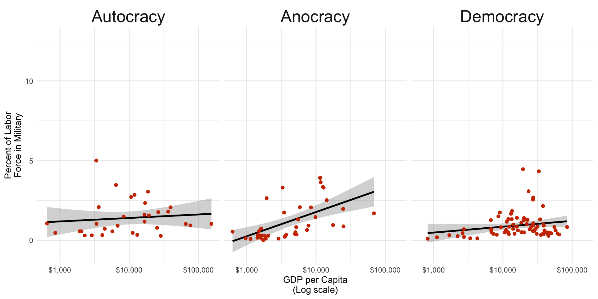
ggplot(aes(y = wdi_afp, x = mad_gdppc)) +
geom_smooth(method = "lm", color = 'black') +
geom_point(color = 'orangered3') +
facet_wrap(~type) +
scale_x_log10(labels = scales::label_dollar()) +
theme_minimal() +
theme(strip.text = element_text(size = 20)) +
labs(
y = "Percent of Labor\nForce in Military",
x = "GDP per Capita\n(Log scale)"
)Introduction to R: Basics
Kevin Reuning
Who am I
- I’m Kevin Reuning (ROY-ning).
- I’m an Associate Professor in Political Science.
- Prior to grad school I had very little experience in coding.

Goals For this Bootcamp
- Not be afraid of R/Rstudio
- Able to load data in and calculate useful statistics with it.
- Difference of means and linear regression.
- Make a variety of beautiful plots.
- Exporting reports using Quarto
Where We Are Going
Where We Are Going
Goals for Today
- Start using R and RStudio, realize you cannot break it.
- How to use R as a calculator.
- Understand the basics of variables and functions in R.
- Load data into R and calculate the average of different variables.
R and RStudio
- R is a statistical language used to do analysis.
- R is free.
- R makes it easy to create reproducible analysis.
- RStudio is an interface that sits on top of R and makes life easier.
Following along
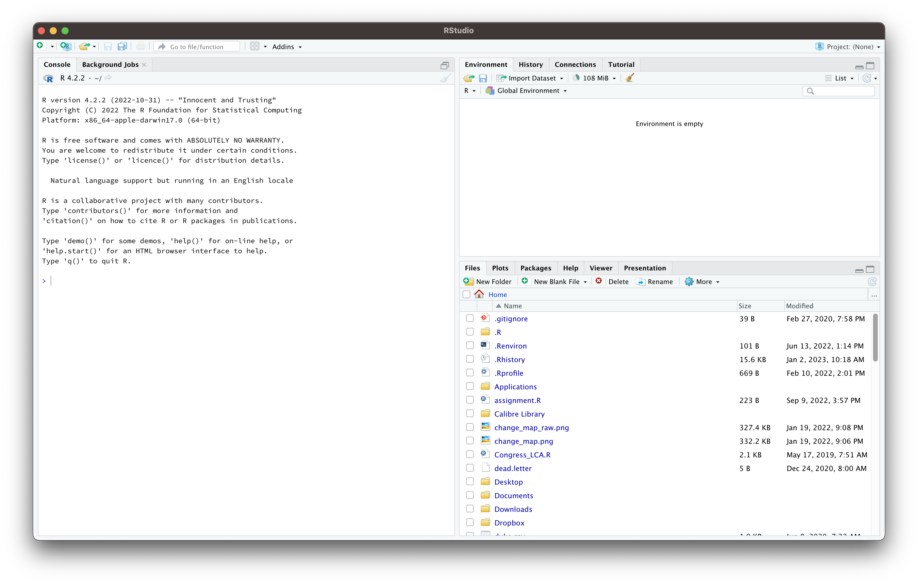
You need to learn by doing. If you haven’t opened RStudio yet, do so now. You should have something like:
Rscripts
- R Scripts allow you to save and re-run everything you did to your data. This is incredibly helpful.
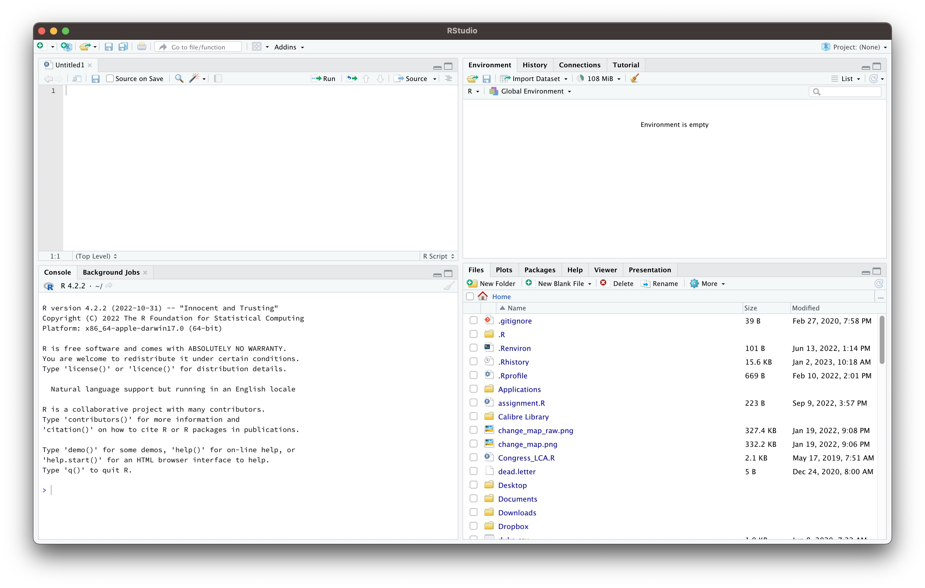
- To start a new R Script: File \(\rightarrow\) New File \(\rightarrow\) R Script.
- When you are done you can save the R Script.
Rscripts in RStudio
You should now have 4 panes.
Running things in R/RStudio
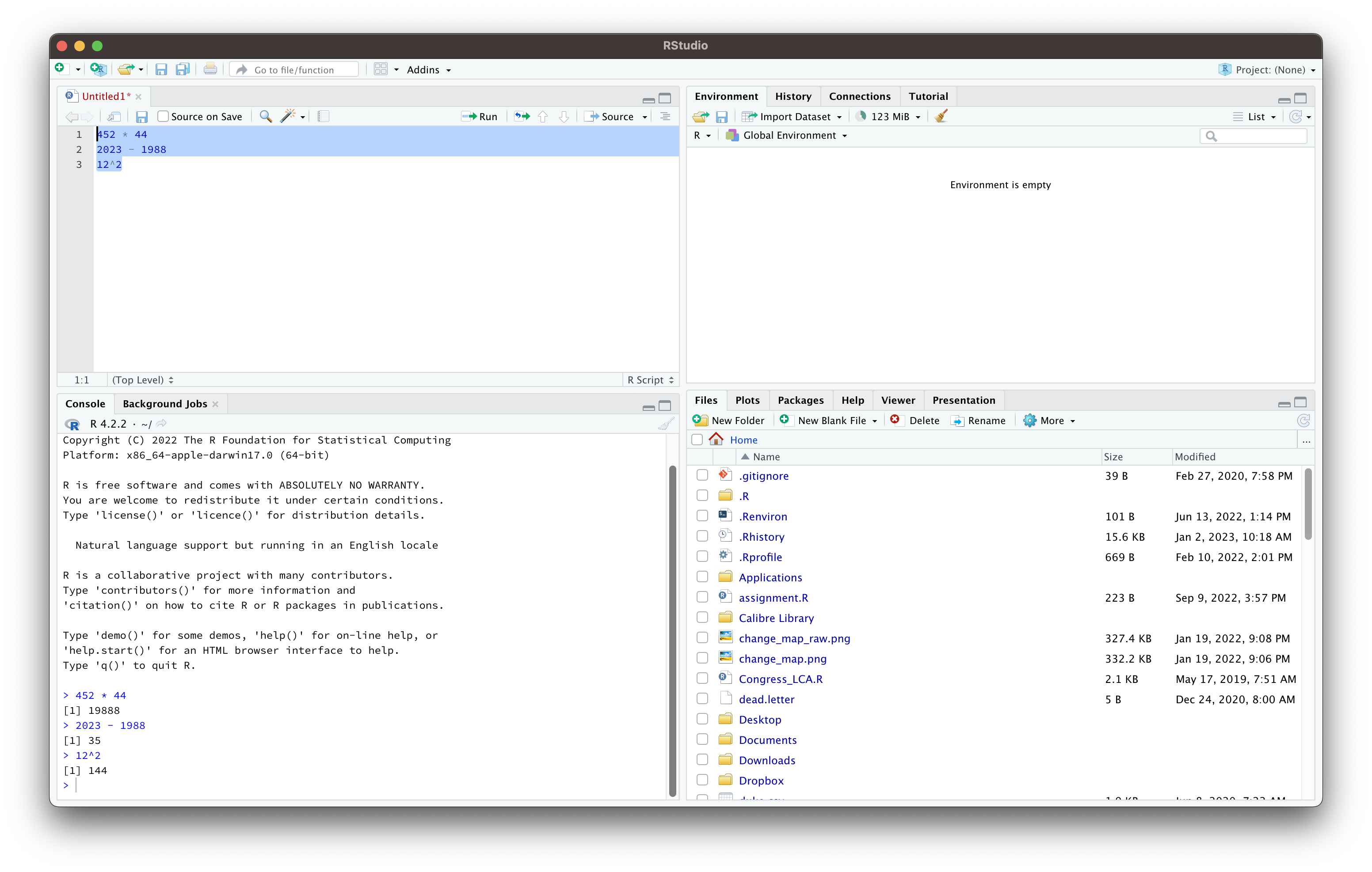
To run parts of your script in R you have to two do things: 1) indicate what you want to run, and 2) tell RStudio to run it.
- Indicating: In the Script part of the Window you will highlight large blocks of code or leave your cursor on the specific line you want to run.
- Running: Click the button that says “Run” to the top right of the script window. Or hit Ctrl + Enter (Windows) or Command + Return (Mac)
Notes about Slides
Throughout this I will show you code and the output in R (Note: You can leave comments to yourself using “#” and R won’t run that line).
[1] 1The output will be immediately below it. This should be similar to how you’ll have code in the RScript pane and the results in the pane below.
R as a calculator
R can be used to add, subtract, multiply... Type something similar in the RScript pane, highlight it and then click “Run”
[1] 3[1] -1[1] 30[1] 2.333333R as a calculator
You can also exponentiate things and even access special numbers such as \(\pi\)
[1] 25[1] 3.141593[1] 6.283185General Advice
- The hardest part of learning to code is that there are lot of rules but also a lot of flexibility. Sometimes you have to be very precise and sometimes you don’t.
- You’ll learn these rules as you try different things. Don’t be afraid to try to break R.
- You can (and should) save scripts so you can re-run and change things. Every R script should be a self contained world.
Spaces
Spaces (or not) between things often don’t matter
Check
At this point you should have RStudio open, and be able to type things in the RScript pane and run it in the console pane below. Your screen will look something like this.
Variables
In R you can store information in order to retrieve it later. These are called variables.
You use an arrow <- (less than and dash) to save a value as a variable.
Variable Names
You can name a variable almost anything with numbers, character
Rstudio and Variables
One of the benefits of RStudio is that it will show the stored variables in the top right pane.
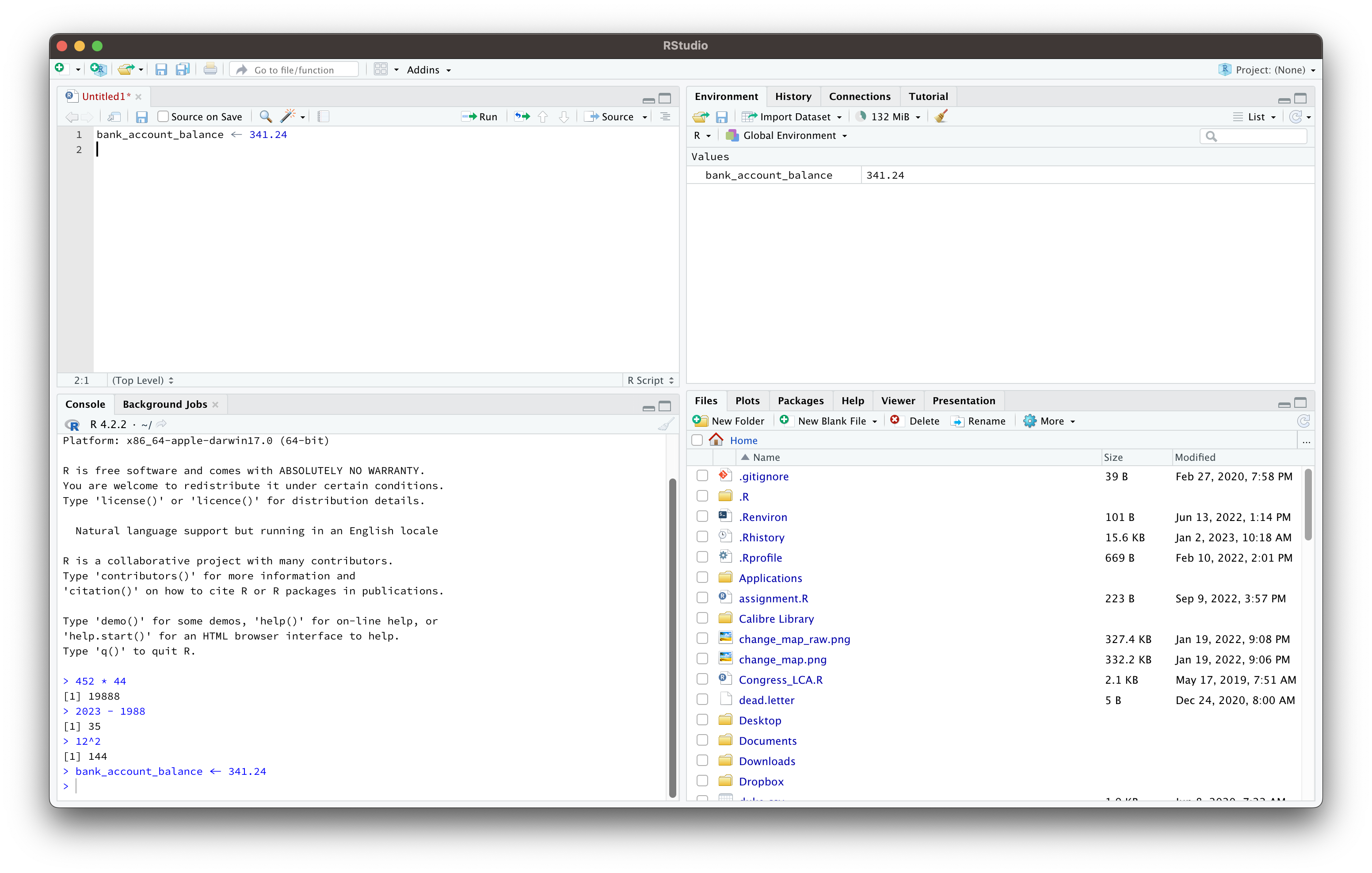
Here I’ve saved the number 341.24 to the variable bank_account_balance
Overwriting Variables
There is nothing stopping you from saving on top of the variable with a new value.
Types of Variables
There are two base types of variables you can use:
- Numeric/Doubles: These are just numbers. You don’t include a commas just numbers.
- Strings: This is anything as long as it is surrounded by
" "(quotation marks). - Factors: This is a combination of the two and we’ll discuss it more later.
String Examples
Vectors
You can also store a series of numbers or characters. This is called a vector
- To store a vector you surround everything with
c( )and put commas between each item in the vector. - Everything in a vector has to be the same type (all numbers or all strings)
Vectors Examples
[1] "Kevin" "Claire" "Mike" "Dominick" "Leona" [1] "Kevin" "34" "Claire" "23" Warning
If any item in a vector is a string then R will make everything a string.
Vector Math
You can do math on vectors
Check
Using R as a calculator, calculate the volume of a sphere with a radius of 2 and store that value as the variable vol
- You can do this all in a single line.
- The formula is \(\frac{4}{3} \pi \cdot \text{r}^3\)
- Then use a vector to calculate the volume of 3 different spheres with radii 3, 6, and 8.
How I did it
Functions
Functions in R take the form of function(X, Y, Z) where function is the function, and X, Y, X are a bunch of arguments that give the function an input and/or tell it what specifically to do.
Additional Arguments and Missing Data
sum() has an additional argument that you can use to tell R what to do with missing values. First, how does R no a value is missing? These are recorded as NA.
[1] 147.6 52.8 38.4 80.4 NAsum() has a second argument na.rm that tells it what to do with missing values. If we want to ignore them we need to set this argument to TRUE:
na.rm is a logical argument. It can either be TRUE or FALSE and so acts as switch. If TRUE then missing values are ignored, if FALSE (the default) they are not ignore and so a missing value is returned.
Accessing the Manual
R has a manual for each function. These are a good place to look if you don’t know what arguments a function has, but they can take practice to read.
You can access the manual by typing ? followed by the function name in the console: ?sum
The manual itself will appear on the bottom right pane.
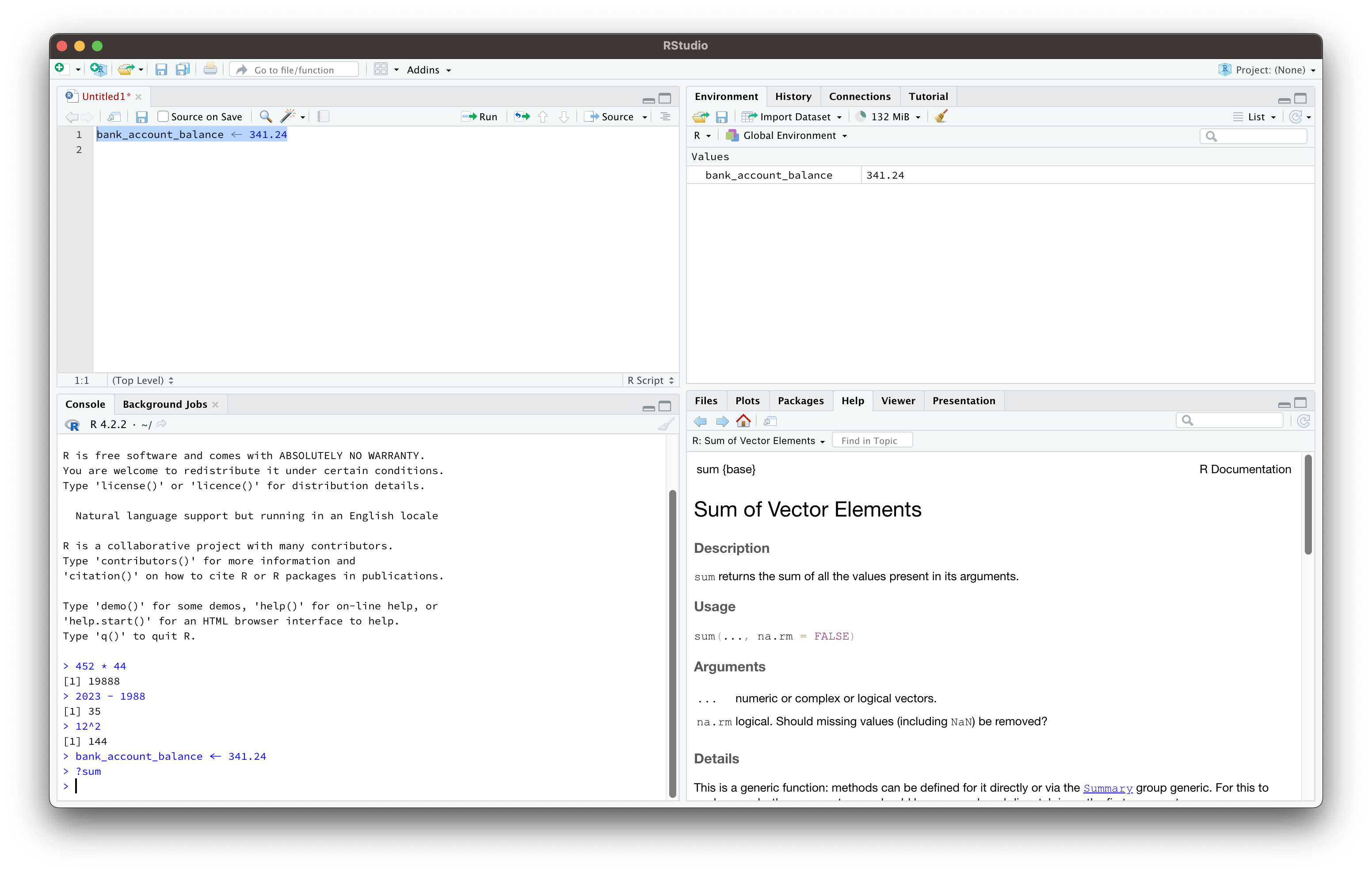
Reading the Manual
The manual can be hard to read at first. A few tips:
- The Description is often very general (to a point of sometimes not being useful).
- The Usage shows all the arguments and their defaults (if they have any). There is more info about the arguments in the Arguments section
- At the very bottom there is usually an Examples section. You can often copy these into the script pane, run them, and see what happens.
Some Other Functions:
mean()median()sd()range()
Take a moment now, and look at the manual of one of these functions.
Libraries
- R is powerful/useful because anyone can extend it (add more functions).
- Bundles of functions are called libraries/packages.
- You can install a library with
install.package()and then tell R you want to use it withlibrary.
Tidyverse
- A lot of data science work is done using the Tidyverse suite of packages.
- We can install the entire suite using:
install.package() - We are going to install a few other packages we will use during the bootcamp now as well.
Run:
There might be a popup asking about installing things from “Source” you can hit no on it.
Using a Package
- To use a package you use the function
library(). - It is a norm to load all the packages you use in a script at the top of a script.
Loading Data
readris a library used to load datasets.- We are going to start with loading it using RStudio’s interface.
Download this data and we are going to open it in R. It has data on the number veterans in each county receiving disability benefits.
Importing Data with RStudio
- In the bottom right you can look through files, it shows the working directory.
- You can change the working directory by going to Session \(\rightarrow\) Set Working Directory \(\rightarrow\) Choose Directory…
- Find ‘disability_comp.csv’, click on it and select ‘Import Dataset…’
- The first time you do this there might again be a popup asking you to install something, click “Yes” on this one.

Importing Data with just R
We can do the same thing but just using R:
Note
Mac computers file paths start with ~/ and Windows start with C:/.
If you write setwd("C:/") you can then hit tab and walk through the folders.
Looking at your data
Once you have the data loaded start by just running the data by itself. It will show you the first 10 rows of data.
# A tibble: 3,142 × 9
    FIPS State   County   Total Age_under_44 Age_45_65 Age_over_65  Male Female
   <dbl> <chr>   <chr>    <dbl>        <dbl>     <dbl>       <dbl> <dbl>  <dbl>
 1  1001 Alabama Autauga   2000          466       957         576  1687    313
 2  1003 Alabama Baldwin   5073          936      1553        2584  4648    425
 3  1005 Alabama Barbour    605           97       242         266   537     68
 4  1007 Alabama Bibb       278           56        95         127   252     26
 5  1009 Alabama Blount     771          159       217         395   724     47
 6  1011 Alabama Bullock    152           22        67          63   133     19
 7  1013 Alabama Butler     414           82       168         164   362     52
 8  1015 Alabama Calhoun   3228          540      1177        1511  2847    381
 9  1017 Alabama Chambers   663          127       201         335   601     62
10  1019 Alabama Cherokee   419           59       124         236   395     24
# ℹ 3,132 more rows
Accessing individual columns
To access a specific column of data you’ll use the $: data$column.
[1] 2000 5073 605 278 771 152 414 3228 663 419 736 241
[13] 485 269 190 2853 1071 274 239 862 290 1345 2629 879
[25] 831 2659 735 1857 314 293 720 159 277 413 2696 724
[37] 10724 222 1574 382 3999 2257 230 532 11686 428 398 1444
[49] 8234 440 7674 1857 147 10 372 706 420 3191 1385 2970
[61] 210 1482 1028 3658 1078 241 157 379 NA 35 10388 91
[73] 18 65 43 4954 49 38 502 1426 255 383 28 16
[85] 3760 66 34 33 57 111 138 14 259 194 47 NA
[97] 44 753 7481 1871 1070 424 122 582 65815 5434 1751 22491
[109] 8370 451 5800 4695 234 271 999 3714 622 146 70 445
[121] 149 313 264 566 116 296 374 1373 1108 690 254 116
[133] 173 256 2023 293 295 1928 291 757 278 496 171 518
[145] 285 198 1229 393 97 220 92 162 219 386 2342 248
[157] 371 659 614 137 204 141 128 454 188 245 169 303
[169] 437 984 105 9963 353 328 2008 185 158 2228 175 441
[181] 260 545 435 3099 1405 112 292 11666 13 792 3317 919
[193] 202 10439 565 3013 11678 325 2058 2106 335 12071 3942 1453
[205] 607 71255 1928 1709 376 1280 2840 179 156 6132 1766 119
[217] 1862 26528 6221 490 37114 21131 751 28457 88830 5178 7758 4024
[229] 4691 5780 11221 2163 3763 44 897 12346 5173 5393 1807 1093
[241] 239 5181 1097 10180 2307 2291 6371 236 10544 301 45 141
[253] 3047 895 382 25 144 125 114 91 233 741 8391 38
[265] 4903 333 490 38877 1297 701 81 230 224 22 189 23
[277] 8038 19 84 138 728 5690 353 81 309 3865 25 249
[289] 605 876 323 364 87 492 51 116 204 4239 131 248
[301] 271 93 15 79 52 295 1023 59 4235 87 5456 8558
[313] 1908 1754 8088 5033 1531 1573 5132 6105 3762 7677 4667 490
[325] 7895 486 18197 20468 237 4513 4243 8184 4356 1802 509 341
[337] 26484 13312 2547 251 823 364 293 449 295 278 464 4914
[349] 2416 30498 468 3214 1045 254 92 8189 12219 4486 1020 118
[361] 344 6603 8130 2421 18968 2423 2106 15263 759 21034 6432 15807
[373] 12405 19698 12519 1619 5073 5896 8960 7258 7691 3611 966 428
[385] 216 12801 596 2202 645 269 105 139 58 814 231 1077
[397] 1713 298 430 3550 251 294 317 1955 1224 501 390 113
[409] 2689 164 1679 1037 227 9400 996 419 3531 1560 86 6469
[421] 99 11078 597 597 7380 345 2651 264 328 268 408 418
[433] 11634 328 165 2518 2935 179 39 1676 310 351 181 612
[445] 2453 1350 2082 294 14877 653 44 1920 717 323 316 10884
[457] 652 2593 237 381 1236 368 171 6085 8660 131 1110 240
[469] 208 313 124 143 497 322 291 1132 824 7691 219 1172
[481] 3648 593 485 318 208 454 213 414 81 321 493 113
[493] 306 448 11126 2122 439 235 2790 839 540 335 322 647
[505] 208 434 72 333 138 9520 2090 65 222 137 1203 432
[517] 106 517 195 26 521 147 172 188 812 648 424 349
[529] 98 1390 173 182 769 442 1076 1360 686 101 354 659
[541] 38 98 551 1016 116 222 178 380 3230 27935 NA 1158
[553] 2068 8775 116 1481 84 256 572 182 302 1149 1546 309
[565] 49 14 3619 100 213 NA 241 89 1946 120 227 432
[577] 163 416 314 232 3808 569 193 189 50 223 161 883
[589] 68 188 447 84 323 79 1161 380 218 1064 135 249
[601] 501 67 332 68 213 144 1828 432 225 168 648 608
[613] 32832 254 128 970 207 201 5522 207 74 385 231 166
[625] 794 436 116 161 546 100 308 56 108 643 343 882
[637] 112 636 297 298 217 3285 1135 1054 634 7938 1173 221
[649] 394 379 292 456 2554 1631 1321 672 4074 623 149 189
[661] 260 191 247 445 393 461 166 565 2068 293 192 223
[673] 88 133 61 413 217 1862 8446 411 2535 116 71 272
[685] 60 531 1588 269 1184 139 157 209 200 229 691 5077
[697] 1334 2926 402 333 5253 1135 84 265 699 380 292 702
[709] 2066 460 332 233 381 741 309 767 1782 536 1982 367
[721] 1372 213 338 429 425 1750 602 3645 1306 755 2752 778
[733] 2207 749 490 398 340 579 414 2734 570 921 286 5058
[745] 1221 955 2194 13569 576 229 1295 1717 448 1245 155 722
[757] 85 334 386 277 326 154 1917 335 160 595 336 431
[769] 198 3395 363 623 307 302 603 311 148 1761 276 100
[781] 2461 253 1483 672 103 878 492 979 444 399 528 96
[793] 50 207 217 101 316 1546 493 283 233 231 189 162
[805] 334 257 242 848 201 152 187 61 208 297 558 219
[817] 1164 101 139 181 485 290 1157 147 252 260 155 186
[829] 141 154 224 257 190 246 325 240 153 165 106 181
[841] 282 554 149 1260 287 113 246 475 2527 126 146 155
[853] 304 295 605 535 419 141 178 167 182 464 191 83
[865] 266 169 267 104 6599 1913 237 88 195 2425 254 254
[877] 1020 196 100 212 109 432 888 279 121 685 173 225
[889] 1330 135 193 146 82 254 47 269 186 156 973 37
[901] 52 268 32 26 291 144 124 17 480 442 35 652
[913] 107 1256 27 67 296 94 244 259 330 4726 35 28
[925] 38 49 106 16 50 409 34 21 219 345 54 5872
[937] 31 89 26 222 17 3866 38 176 26 368 314 108
[949] 153 42 391 74 501 135 27 115 143 34 56 316
[961] 32 73 79 91 514 103 42 798 75 126 2529 66
[973] 42 91 800 60 7871 138 3183 28 72 63 46 NA
[985] 33 314 96 50 143 20 80 23 146 44 1857 262
[997] 289 377 129 636 149 373 1755 250 947 417 109 178
[1009] 452 1225 220 211 574 1068 81 130 373 234 5025 625
[1021] 215 156 157 117 1350 203 61 212 3658 196 476 704
[1033] 100 81 288 359 487 458 163 711 132 7136 NA 474
[1045] 266 257 562 196 63 747 167 10030 638 409 1992 192
[1057] 428 286 945 271 111 115 300 197 345 129 434 182
[1069] 1079 322 112 1591 115 230 556 112 213 1513 95 333
[1081] 116 134 411 143 410 731 110 326 784 141 53 220
[1093] 434 783 219 1236 30 253 293 281 690 574 291 265
[1105] 356 241 484 157 207 1755 144 310 177 619 82 347
[1117] 685 322 1448 245 749 1150 222 4510 4837 3073 144 82
[1129] 139 227 313 422 5721 77 275 378 244 440 882 399
[1141] 233 5601 400 3455 875 191 554 1673 149 411 655 5428
[1153] 2370 555 283 3369 85 262 482 539 651 165 265 577
[1165] 1345 692 633 4460 1791 62 1208 328 728 4128 755 616
[1177] 356 130 133 209 2334 1920 4668 660 1087 3387 808 840
[1189] 1190 3390 477 1084 1374 874 975 4035 960 13968 8730 2105
[1201] 394 1882 1715 5278 439 4100 426 5268 4108 232 9562 17527
[1213] 614 4173 322 430 2161 1294 920 6937 3806 1427 6778 191
[1225] 7252 998 5910 1908 13365 63 6594 7346 6390 9447 318 237
[1237] 1065 505 410 299 189 717 1679 338 1840 592 2142 647
[1249] 403 588 869 760 790 405 1022 735 1299 564 5201 566
[1261] 337 1372 624 640 708 569 2859 702 713 346 770 2075
[1273] 2630 374 5792 93 309 1176 317 1321 2020 138 260 9139
[1285] 467 1713 450 619 520 1267 235 1723 843 283 2142 825
[1297] 10728 426 451 252 430 270 491 2281 327 711 2664 2602
[1309] 647 599 239 1003 924 849 2966 17924 555 529 5985 763
[1321] 932 1062 218 1163 603 971 1310 1071 250 1075 1042 225
[1333] 139 263 2104 6730 336 976 325 443 721 962 153 13274
[1345] 391 736 1011 1421 159 486 907 85 375 223 342 104
[1357] 627 96 437 754 69 219 476 657 964 1227 700 164
[1369] 668 250 131 2271 1244 272 812 101 566 292 5839 72
[1381] 350 352 974 131 247 5054 2000 2184 373 4332 584 143
[1393] 209 763 87 542 450 466 3556 253 117 723 2240 240
[1405] 489 531 163 239 70 365 185 141 190 101 132 226
[1417] 268 274 456 272 2684 1723 102 320 148 372 910 8366
[1429] 3658 180 89 10 230 3754 233 84 200 838 146 547
[1441] 1166 1546 216 262 1064 336 438 1688 1416 337 352 521
[1453] 170 307 345 104 562 392 1171 203 635 354 275 103
[1465] 2206 280 56 345 178 386 258 130 344 231 258 158
[1477] 299 177 790 660 236 148 93 241 191 318 385 271
[1489] 94 443 550 164 259 678 212 2929 1353 1165 164 1052
[1501] 1223 1345 138 164 1797 302 158 1500 96 3662 348 1543
[1513] 378 498 128 333 157 176 353 283 460 1332 276 98
[1525] 4603 206 153 536 268 88 215 857 241 9551 1727 3144
[1537] 2109 78 988 589 693 179 804 262 242 283 356 299
[1549] 269 523 91 565 179 264 219 218 608 337 885 289
[1561] 252 261 249 260 311 1033 1337 268 1864 514 4625 81
[1573] 203 528 399 188 303 4734 227 262 1306 10733 417 66
[1585] 74 785 199 130 724 693 82 1160 851 298 524 371
[1597] 313 679 38 411 3911 193 136 110 168 232 15 3546
[1609] 95 222 27 149 227 42 204 2151 1719 21 209 24
[1621] 74 339 373 67 578 2051 23 603 17 186 50 141
[1633] 2117 131 311 11 68 88 23 159 32 1198 143 139
[1645] 143 387 45 655 194 83 137 113 12 159 40 NA
[1657] 3054 742 172 NA 25 NA 159 226 52 74 1070 135
[1669] 208 1010 171 53 101 298 159 158 161 293 346 187
[1681] 371 63 922 8931 35 187 140 59 154 706 46 80
[1693] 89 15 81 1634 299 123 17 75 231 NA 240 193
[1705] 84 128 201 12 83 277 5947 812 15 24 NA 577
[1717] 290 119 101 138 135 368 61 45 267 108 677 162
[1729] 295 199 28 258 7938 593 832 484 113 124 16 91
[1741] 141 23 131 342 155 95 14 526 1198 44181 1049 798
[1753] 17 34 245 91 93 1579 127 1770 92 109 8243 173
[1765] 1156 1277 1092 1214 748 1529 6390 2479 4643 2151 849 2766
[1777] 4525 7542 4840 1751 1282 4669 3142 3093 794 2449 4422 4756
[1789] 2677 6527 2430 715 1767 1249 3081 966 14054 109 937 387
[1801] 280 1828 42 4237 772 606 98 21 73 635 547 266
[1813] 370 795 126 3054 219 551 365 3305 1550 555 2315 348
[1825] 287 661 326 74 1582 3002 856 6491 2003 1520 978 2020
[1837] 1355 653 1549 649 598 604 2644 11653 696 768 697 858
[1849] 642 86 824 6052 9941 485 753 825 7054 653 7178 8078
[1861] 2969 3413 5020 1533 4268 559 1654 778 720 8806 1806 2765
[1873] 1757 1791 2940 1481 460 292 478 1755 10549 920 628 661
[1885] 1728 951 855 1228 5086 573 383 2278 544 220 362 481
[1897] 375 1026 336 680 4369 4223 1502 3240 1259 423 2923 372
[1909] 2460 858 796 286 294 1572 1107 5342 26300 986 749 2194
[1921] 577 1105 4354 954 5520 1022 3417 267 148 919 305 7440
[1933] 1028 5417 1447 1868 381 3193 83 2541 748 3632 368 1518
[1945] 1413 1099 878 923 346 439 13437 276 458 3542 1670 4731
[1957] 400 16747 1355 385 1389 1822 406 561 3312 334 1921 1023
[1969] 2481 1306 2618 1149 1193 718 825 662 1018 285 555 63
[1981] 2454 644 14209 343 252 795 4683 992 1587 538 388 43
[1993] 223 82 16 141 36 33 1517 3046 58 74 48 67
[2005] 37 49 42 31 1705 31 58 42 23 71 20 131
[2017] 31 208 195 141 519 153 78 36 126 64 196 107
[2029] 83 251 144 74 16 37 NA 460 47 342 40 181
[2041] 147 2428 57 571 459 1299 729 1624 885 516 1122 684
[2053] 4892 395 528 2389 2906 712 1595 547 571 14782 607 695
[2065] 1707 1024 2140 431 14086 539 516 921 4928 667 8615 797
[2077] 401 232 334 708 460 223 766 607 1036 781 3153 1096
[2089] 3015 656 3750 4481 459 2902 763 2004 427 494 1517 216
[2101] 10126 313 495 1183 234 732 262 464 900 626 1960 563
[2113] 330 1874 1545 841 1363 661 574 4525 5935 3055 1373 717
[2125] 385 222 2727 1057 1182 586 1404 240 379 94 351 68
[2137] 317 155 1115 599 3312 1009 1151 376 29 8428 110 9776
[2149] 216 358 1483 445 980 67 64 1482 731 1281 68 157
[2161] 59 59 371 345 1463 121 273 825 254 240 331 1158
[2173] 942 977 189 1212 671 823 106 434 927 378 2221 202
[2185] 219 266 20326 1052 958 758 437 1299 1451 832 1983 386
[2197] 58 2198 568 1114 1413 156 169 11668 1727 1111 170 129
[2209] 333 514 1353 6172 989 1312 2008 726 833 3826 3998 59
[2221] 219 209 357 5348 568 2356 2205 312 7253 1514 3091 436
[2233] 5293 202 9120 1629 66 777 1497 562 228 566 8023 47
[2245] 1635 1280 12380 872 2143 737 3696 2173 970 5181 2397 2293
[2257] 107 987 1669 4398 498 1254 830 828 1518 4202 3601 4692
[2269] 440 4177 1787 154 2249 150 496 684 1027 621 203 2788
[2281] 4554 1032 2080 3019 4649 1678 778 1385 537 2189 6474 253
[2293] 2713 1266 652 14375 914 389 1963 359 1076 121 594 831
[2305] 369 839 891 2455 874 4131 385 5251 639 2712 2220 7124
[2317] 1925 510 3706 173 3208 302 364 5584 7562 332 9359 825
[2329] 506 766 947 919 1171 495 5312 537 477 2653 1305 7088
[2341] 1179 404 8505 621 2124 1410 1336 337 6282 285 699 501
[2353] 646 1452 1883 1729 15632 330 4527 5598 477 698 4187 46
[2365] 226 43 103 438 557 72 38 217 19 143 45 223
[2377] 420 51 339 353 117 78 70 39 51 427 33 151
[2389] 92 17 90 57 105 12 283 118 23 34 35 NA
[2401] 89 281 656 873 48 102 43 60 1220 21 32 3642
[2413] 99 143 4258 55 43 171 26 98 65 26 92 69
[2425] 166 269 104 371 13 1647 657 348 205 2833 1571 921
[2437] 201 481 1411 757 260 579 134 927 1089 224 1469 8908
[2449] 247 269 904 580 598 367 840 821 510 405 1428 250
[2461] 1126 5365 117 390 494 1279 286 376 741 355 220 412
[2473] 186 1177 431 7653 68 329 697 218 605 1107 1050 432
[2485] 276 1609 442 508 1344 232 880 16702 110 429 501 330
[2497] 170 126 291 1209 573 1118 1230 5268 344 292 2306 13790
[2509] 272 731 3296 2911 1406 126 452 339 100 561 3327 251
[2521] 487 433 2205 2248 837 162 1518 785 158 33 1164 373
[2533] 63 891 1640 83 553 30501 67347 236 NA 394 2061 5750
[2545] 2912 186 19 140 778 335 1014 693 423 349 6894 198
[2557] 101 675 39 617 641 90 278 24 65 169 10803 44
[2569] 300 6076 237 47 591 6693 13 47 29 69 23 79
[2581] 26317 122 126 100 10955 377 44 134 65 169 338 1515
[2593] 42 3064 23896 561 379 782 339 75 86 16 7477 158
[2605] 348 180 127 5698 52 561 10 141 256 276 2414 1824
[2617] 457 8130 354 50 145 31 74 959 49804 1073 39 79
[2629] 3818 39 1371 9667 773 259 1232 492 408 732 136 1771
[2641] 309 20 99 198 608 39 3781 91 713 2753 332 197
[2653] 2101 1224 NA 10 1517 72 120 839 33 941 153 1523
[2665] 79 318 279 334 1189 400 29 164 541 NA 4569 55
[2677] 133 5641 20 169 258 49 53 603 478 1569 28 1967
[2689] 482 86 96 385 8732 170 265 22 1011 795 215 264
[2701] 8844 77 45 1667 525 316 2890 73 177 1487 1784 69
[2713] 261 2474 26 80 230 101 201 10 270 1738 185 690
[2725] 317 172 526 1788 83 28 173 48 282 11 3414 157
[2737] 346 145 NA 14 43 89 31847 4591 26 120 18 325
[2749] 3180 15772 361 404 684 37 495 1423 906 1679 916 589
[2761] 158 527 2662 554 83 4583 236 293 11095 1706 82 1144
[2773] 881 61 257 157 106 84 607 948 333 30 5983 183
[2785] 91 71 147 854 88 160 132 178 22 26 10125 133
[2797] 291 290 425 1063 319 3603 242 2535 27 4196 386 488
[2809] 474 1725 147 796 145 330 486 466 915 811 538 966
[2821] 672 1402 293 210 456 244 5286 997 84 1285 140 594
[2833] 328 290 237 737 704 439 118 222 6966 220 95 788
[2845] 159 266 686 176 23858 1192 199 444 852 1343 279 1248
[2857] 287 281 382 188 659 1318 4370 828 43 1281 2499 113
[2869] 996 254 215 414 6000 666 251 185 211 694 264 1035
[2881] 263 500 246 297 316 749 291 295 970 426 425 1997
[2893] 14019 510 107 115 1643 380 819 364 388 713 507 378
[2905] 4112 7330 142 215 876 706 949 430 702 461 3547 4857
[2917] 320 85 420 10343 615 109 726 105 410 233 174 902
[2929] 107 8335 385 814 116 1097 626 297 227 9280 11150 87
[2941] 1389 438 3982 179 3108 1753 456 416 3822 22348 293 412
[2953] 447 147 504 3225 1093 1976 8443 97 2219 519 235 946
[2965] 69 1168 1699 4648 777 22109 12307 639 679 1851 333 2063
[2977] 871 652 368 32794 229 2566 239 11664 12086 1417 11706 100
[2989] 1127 3363 535 2731 305 2887 383 330 340 1770 146 213
[3001] 170 1178 135 190 1012 446 409 243 1574 567 1243 3138
[3013] 378 345 590 347 1147 458 482 1693 506 326 1302 390
[3025] 371 776 609 142 115 239 649 1027 2333 565 230 292
[3037] 389 383 126 149 533 792 232 242 124 1614 400 605
[3049] 322 870 383 3206 248 571 479 1060 516 887 291 5134
[3061] 1027 463 1100 733 1444 133 1188 307 685 476 252 293
[3073] 129 456 1047 612 2303 286 2109 168 460 573 1132 1725
[3085] 1027 341 51 9531 1812 733 866 2259 823 161 718 970
[3097] 1137 379 2295 227 1998 336 1590 1151 491 676 1101 328
[3109] 490 477 674 1194 482 1472 3751 818 561 2311 1328 718
[3121] 178 782 285 276 171 617 344 95 198 4312 280 1356
[3133] 48 599 265 855 177 742 156 307 130 209Check
Pick two numeric variables and calculate the mean, median and standard deviation for them.
The functions you’ll need are: mean(), median() and sd().
Tip
There is missing data so you’ll have to use the na.rm=TRUE argument.
How I did it
Total number of recipients:
[1] 1610.01[1] 438[1] 4284.202Total number of male recipients: