Go over different concepts of centrality in a network.
Calculate those measures in R.
Overview of Centrality
Measures of Centrality
Centrality is often viewed as importance within a network.
There are a lot of ways to measure this importance.
When you apply a measure of centrality you need to consider how your measure conceives of what it means to be central.
Two Broad Categories
There are two broad ways of considering centrality:
Nodes are influential by having a lot of connections (and who those connections are)
Nodes are influential by being in a strategic position in a network (e.g. can control flows along the network)
Variation in Measures
Measures of centrality vary in at least three ways:
How they conceive of importance.
How well they work with undirected vs directed networks.
What happens when there are multiple components.
Simple vs Complex Networks
Everything is simpler with undirected networks so we are starting there.
For directed networks you often get measures of both in and out centrality.
For network with weighted edges you have to think about what the weights mean for influence.
Measures by a Nodes Connection
Degree Centrality
Degree centrality is the number of edges a node has.
A node with high degree centrality is adjacent to a large number of nodes.
The number of components within a network isn’t very important
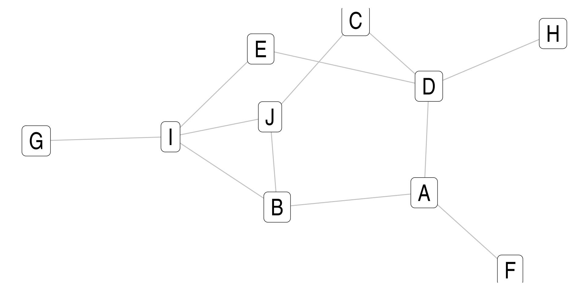
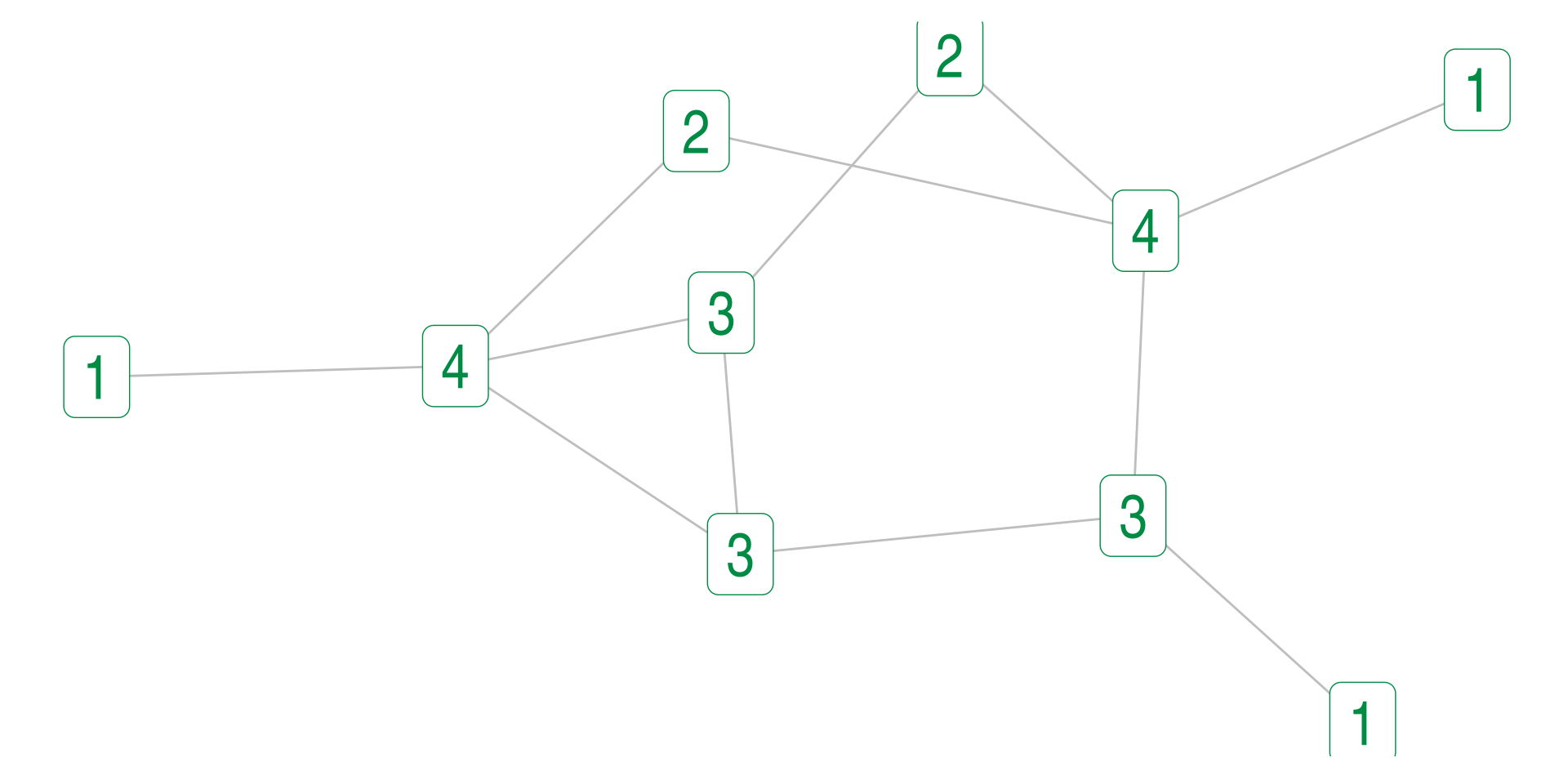
Example
Example
Degree Centrality Limitations
B and F have the same centrality, does that makes sense? Are both of them as important to the network?
Eigenvector Centrality
Our intuition is that how important a node is is a function of the extent of relationships and whether the node it has relationships with are important as well.
What we want to do then is add up how many nodes a node is adjacent to but weight that by how influential each of those nodes are as well.
This creates a self referential equation where the centrality of a node is a function of the centrality of all of the nodes it touches. How do we solve this?
We use things called eigenvectors and and eigenvalues
Eigenvector Centrality
\[ e_{i} = \lambda \sum_j x_{ij} e_{j} \]
The eigenvector centrality (\(e_i\)) of node i is proportional to the eigenvector centrality of the nodes it is adjacent (\(e_j\)). We use the leading eigenvalue (\(\lambda\)) as the proportionality constraint.
Eigenvectors and Eigenvalues
What are these things?
For most matrices \(A\) we can find an eigenvalue \(\lambda\) and an eigenvector \(v\) such that
\[A \times {v} = \lambda {v}\]
In our case we can find the eigenvectors and eigenvalues of our adjacency matrix. There are multiple eigenvalues and eigenvectors but we will be using the eigenvector associated with the largest eigenvalue
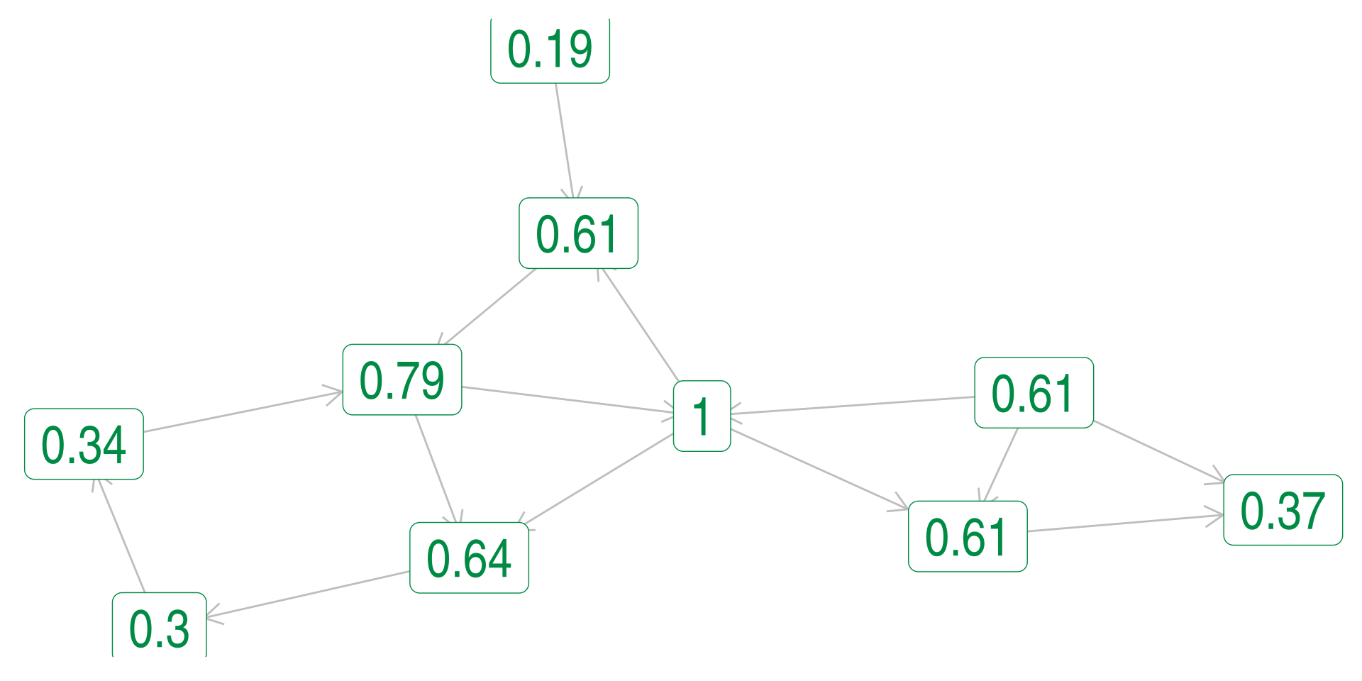
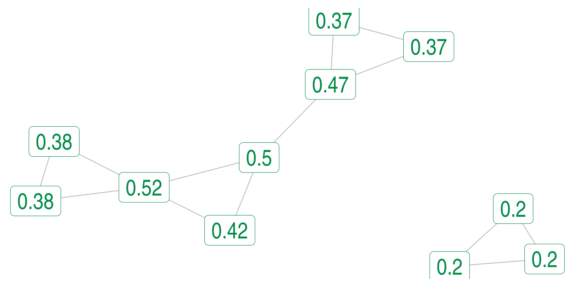
Eigenvector Example
Eigenvector Limitations
Eigenvectors and eigenvalues are only identified up to a proportionality (you can multiply them both by 2 for example and get the same numbers).
To compare across networks we often normalize it so that they sum to 1 or so that the largest is 1.
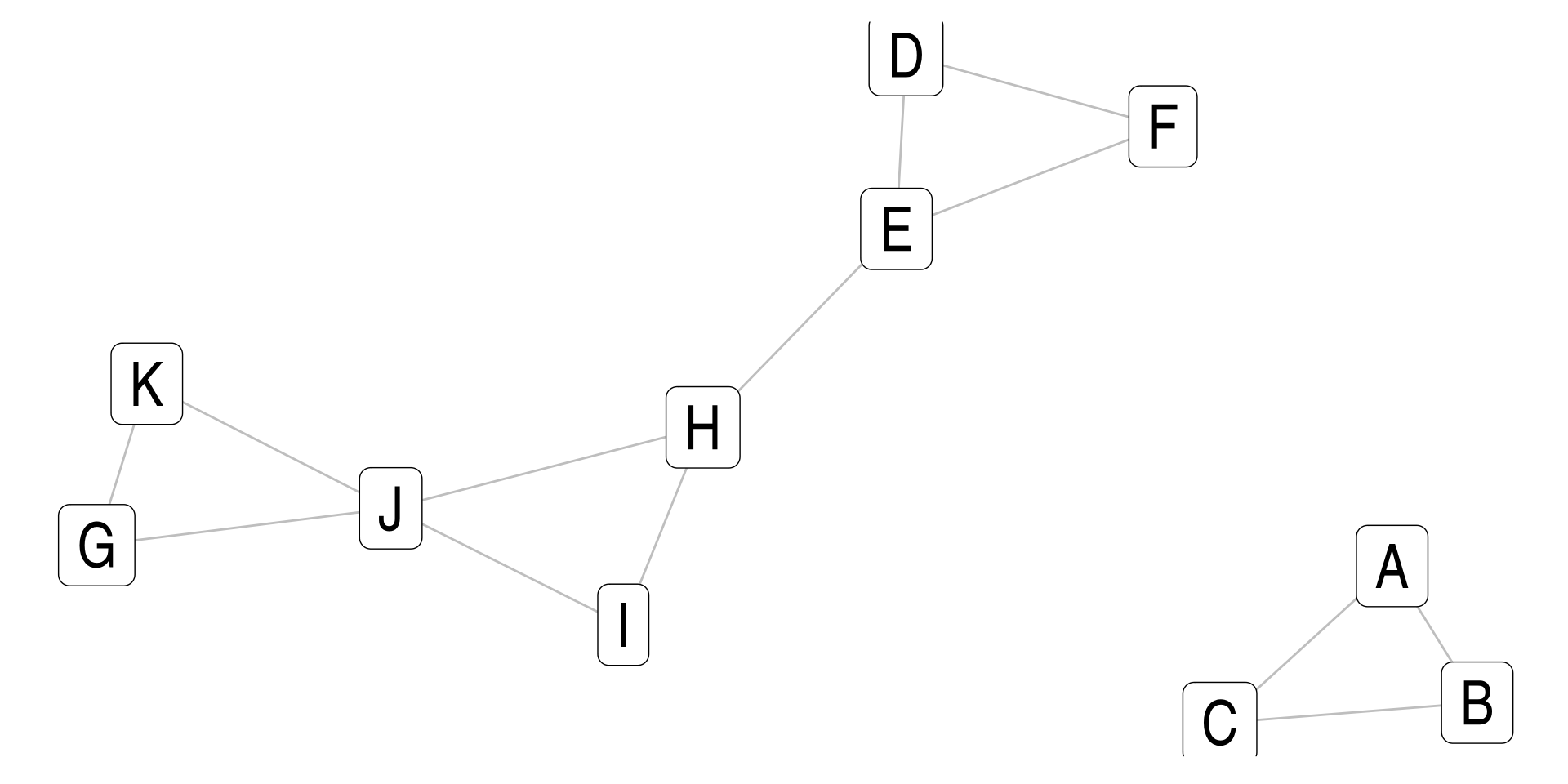
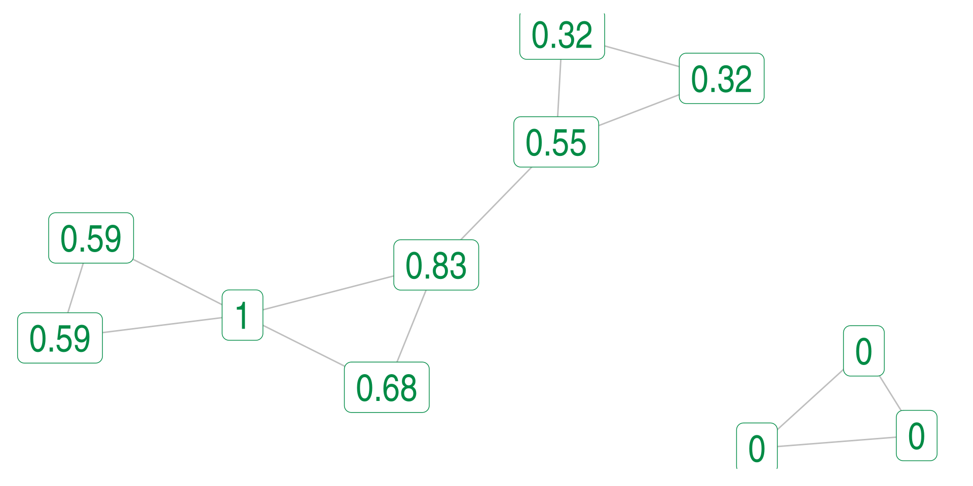
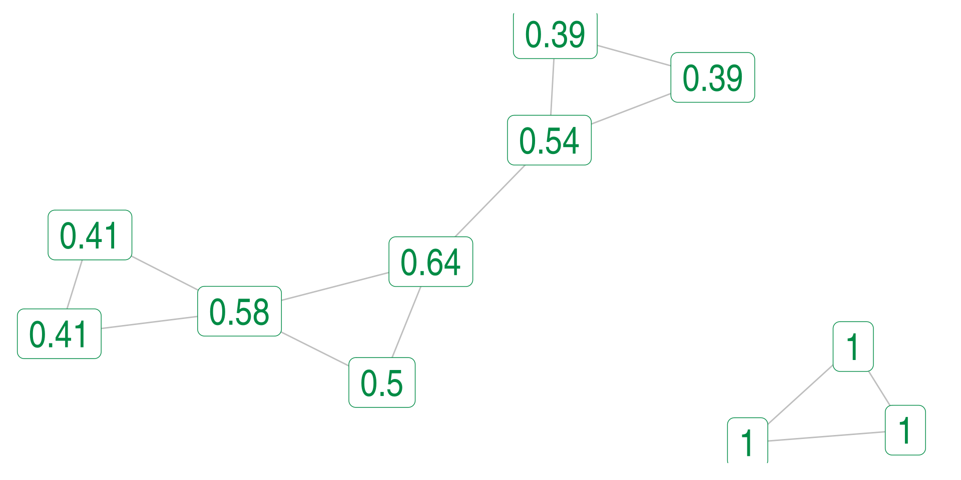
Only vertices in the largest component have non-zero eigenvectors.
Disconnected Example
Directed Network
For both eigenvector centrality and degree centrality the nature of directed networks changes what we mean by centrality.
Degrees and Directed Network
For degree centrality we can divide everything into in-degree and out-degree.
Being high in in-degree centrality can be radically different than being high in out-degree centrality.
In an advice network (“who do you ask for advice?”), having a high in-degree means people often come to you for advice, having a high out-degree means you ask a lot of people for advice.
If it makes sense we can just collapse this into the total (in- and out-degree).
Eigenvector Centrality and Directed Network
With eigenvector centrality we get two measures of centrality. This connects to the fact that we actually have two sets of eigenvectors for a non-symmetric matrix:
Right eigenvectors: Focuses on out-degrees
Left eigenvectors: Focusses on in-degrees
But even with that, these results can get a bit weird.
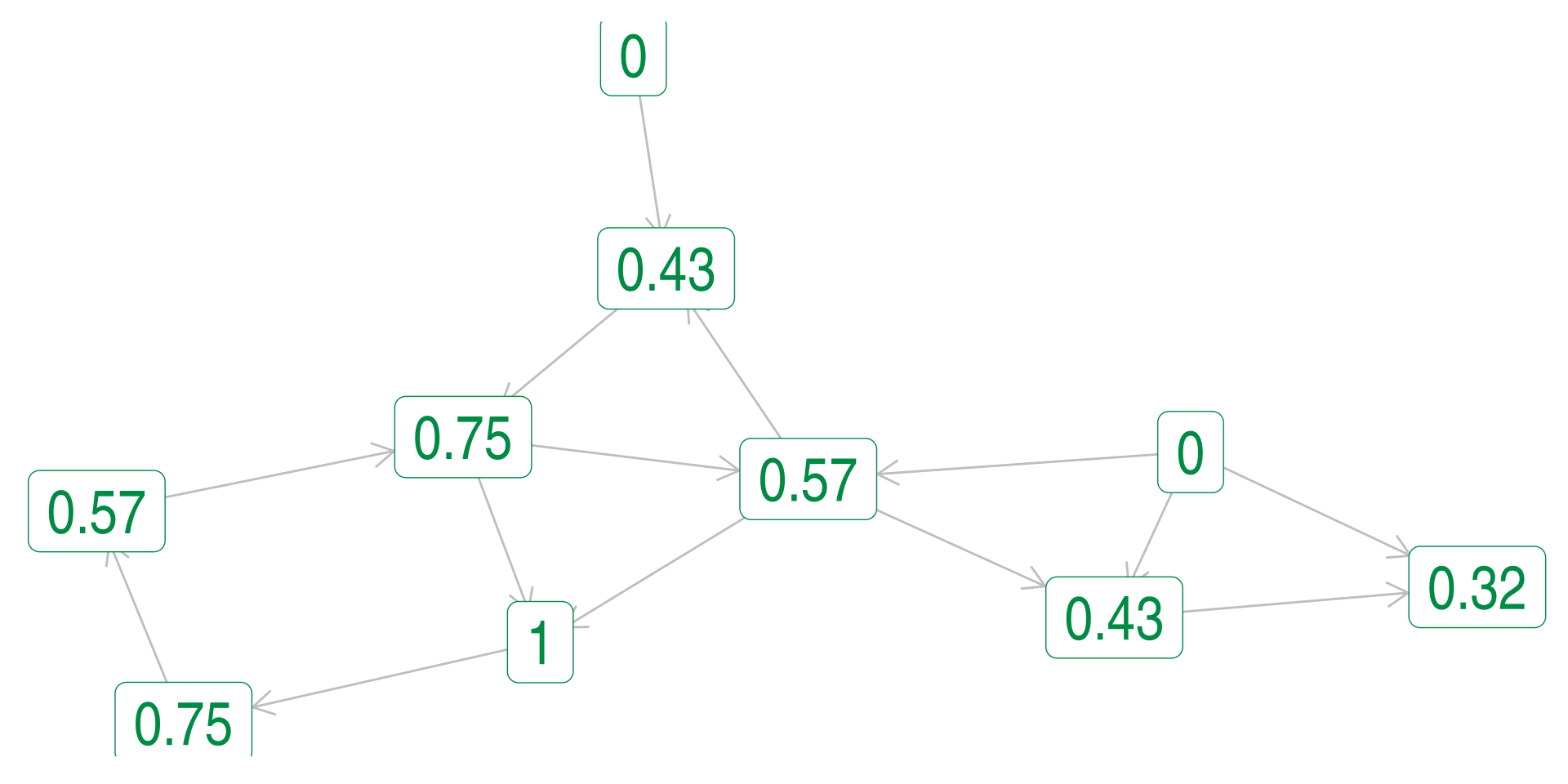
Eigenvector Centrality - In
Using the left or “in” measure of eigenvector centrality:
Eigenvector Centrality - In
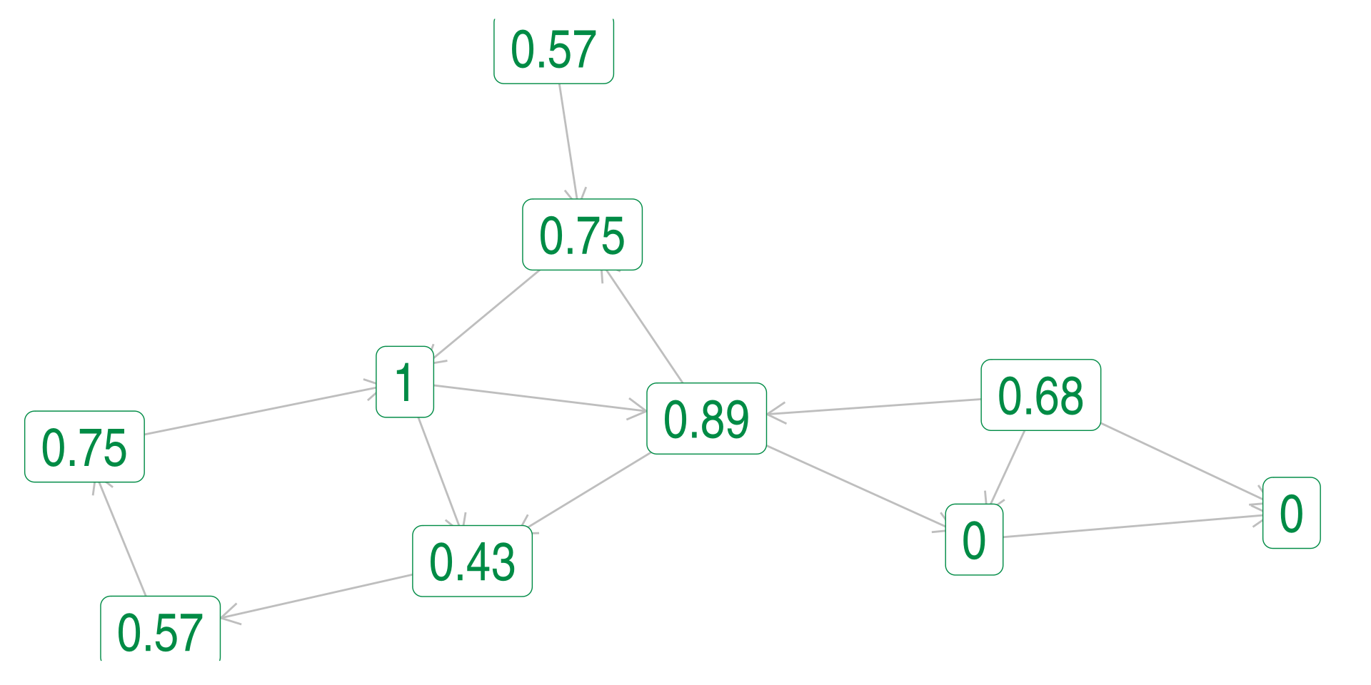
Using the right or “out” measure of eigenvector centrality:
Eigenvector Centrality - Ignoring Direction
We can also ignore the direction of the edges and pretend it is undirected:
Weighted Networks
Finally, for weighted networks the weights can be accommodated easily:
For degree we simply add up the weights (this is often referred to as strength)
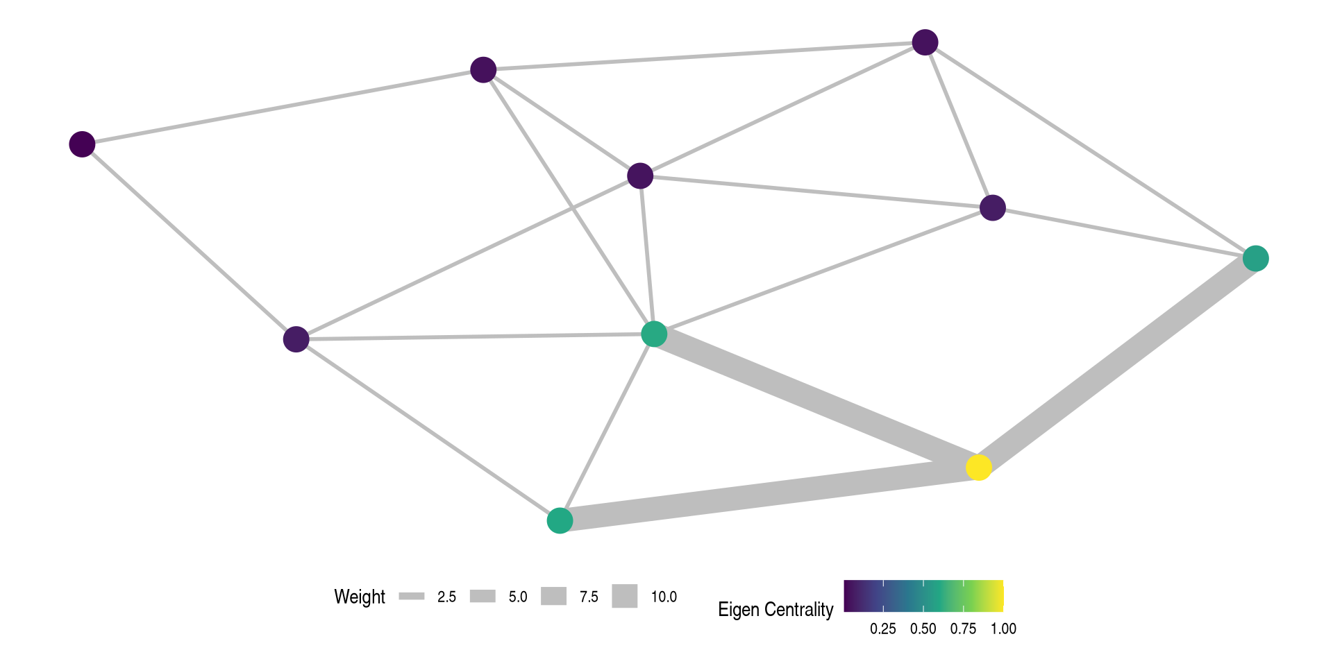
For eigenvector centrality the math does not change, the centralities are now concentrated where the weights are the largest as well.
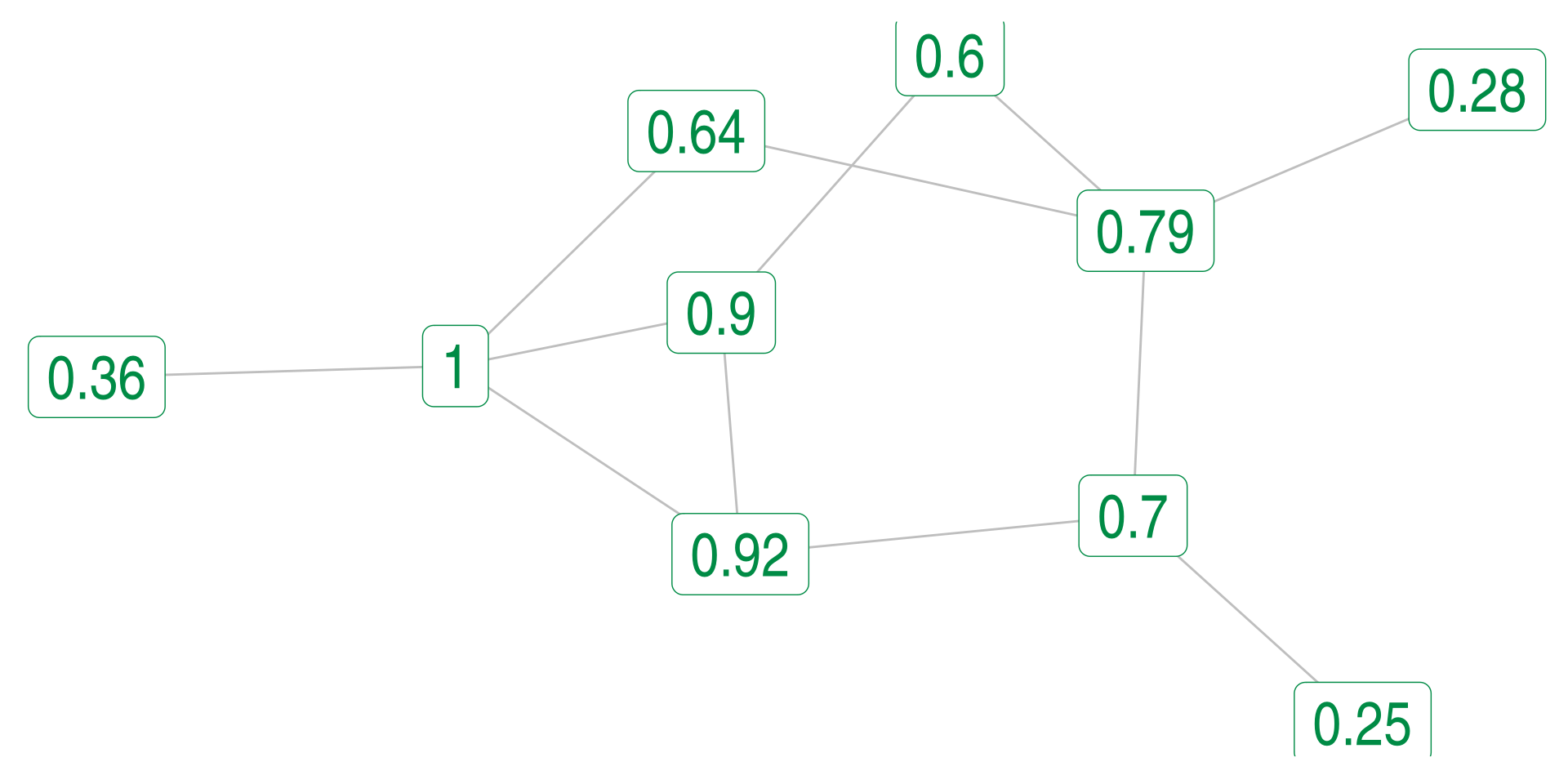
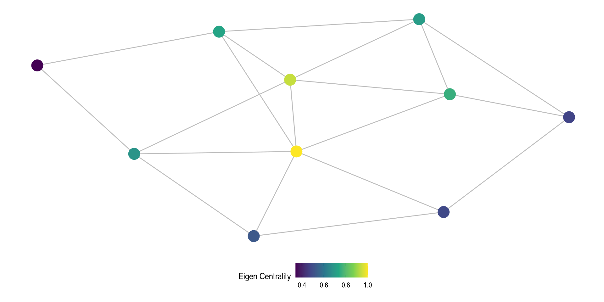
Weighted Eigenvector Example
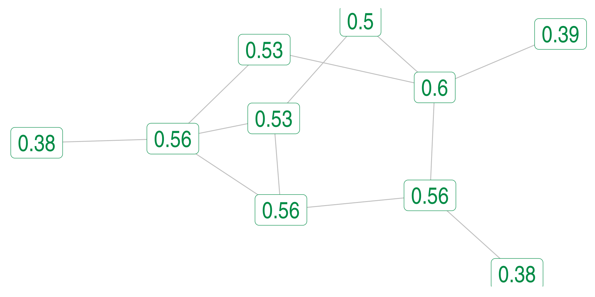
Without Edge Weights
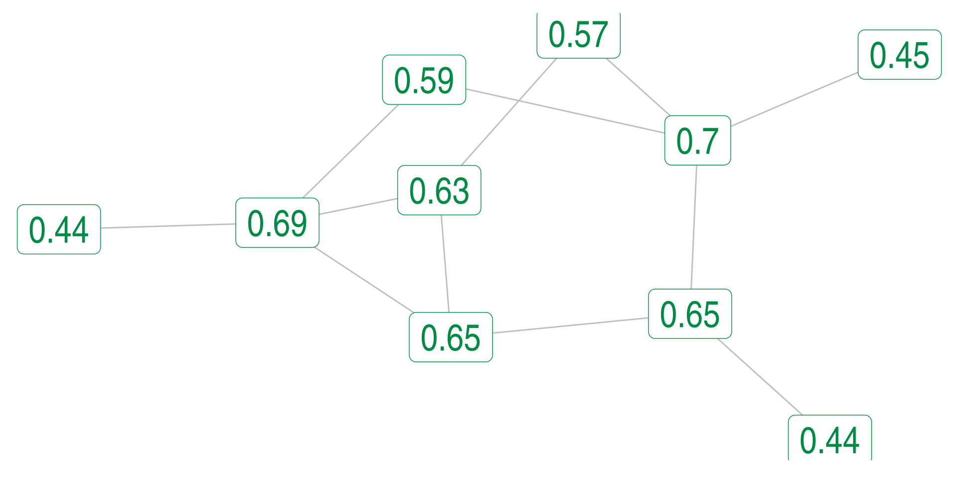
Wth Edge Weights
Calculating in R
The basic functions:
eigen_centrality() Calculates eigen centrality, returns an overly complicated object.
If there is a weight attribute on the edges it will calculate weighted centrality. To turn that off set weight=NA.
Defaults to undirected no matter the network, set directed=TRUE to get the in measure. Transpose your network with t(net) to get the out measure.
degree() Calculate the degree, returning a simple vector.
For directed networks use mode="out" or mode="in" to get out or in degrees.
Ignores weights.
strength() Calculates the weighted degree
Can use mode= for directed networks (see above).
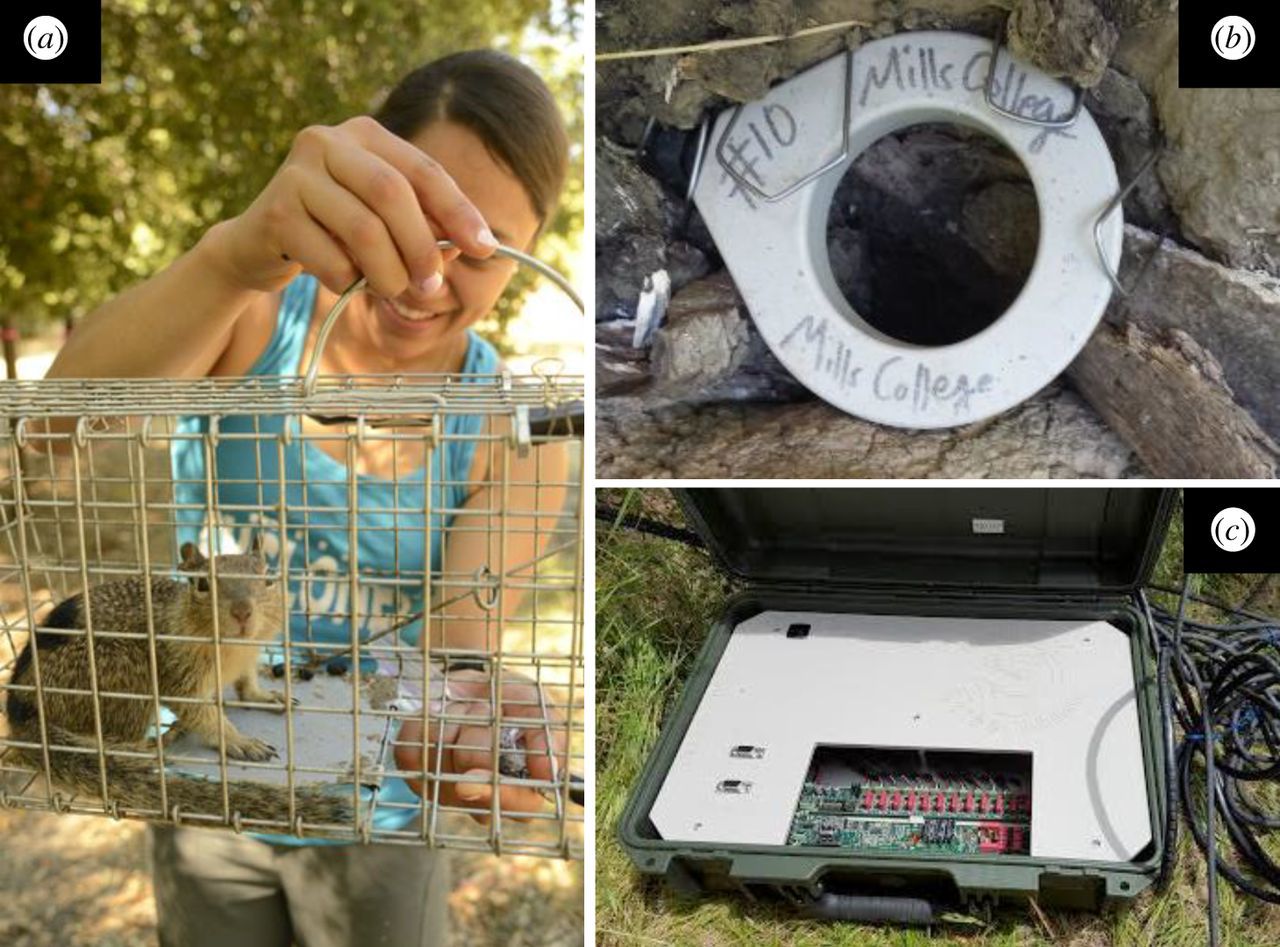
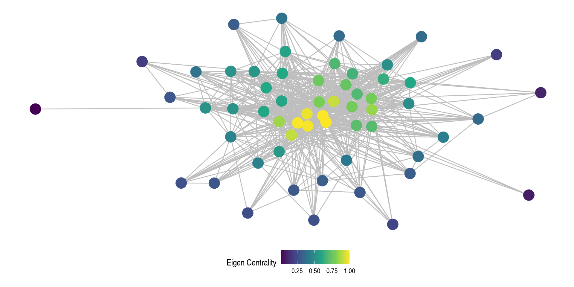
Real Example - Squirrels
Lets use data from a Squirrel burrow sharing network, the data is here with more info here and here
The edges are weighted by the proportion of days they shared a burrow.
Calculating Centrality of Squirrels
We can calculate centrality and then assign the vectors as vertex attributes
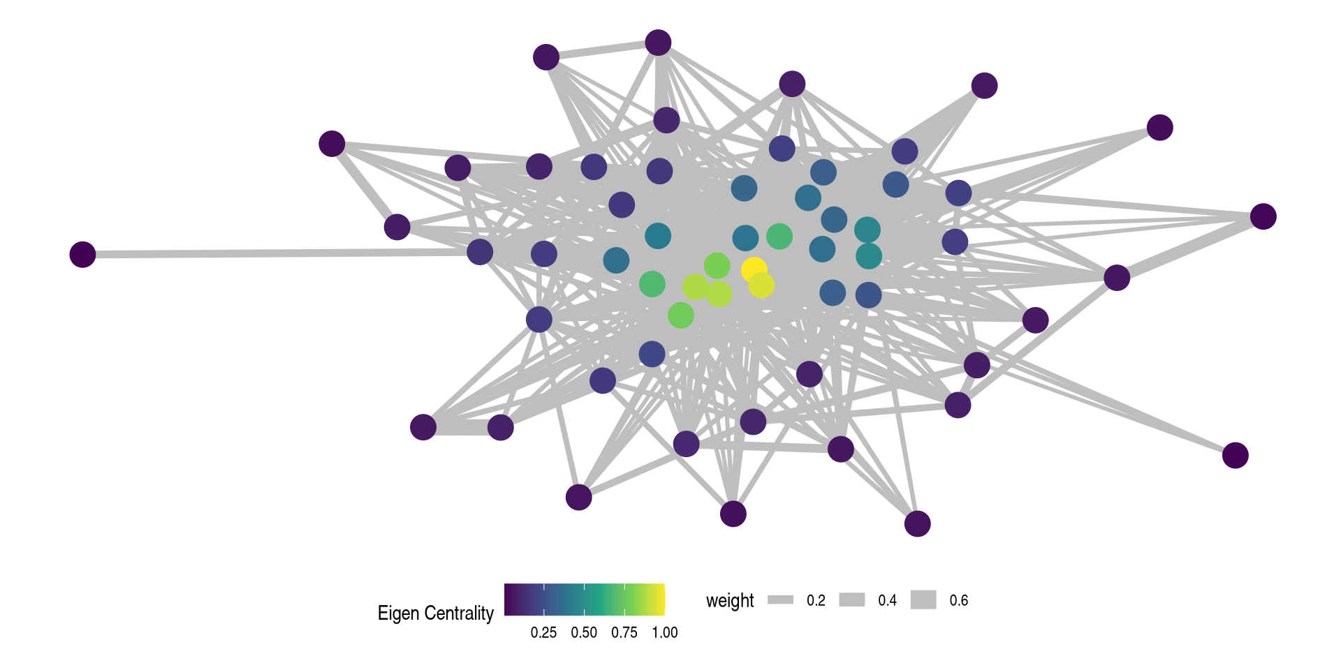
Real Example - Visualizing Network
Unweighted
Weighted
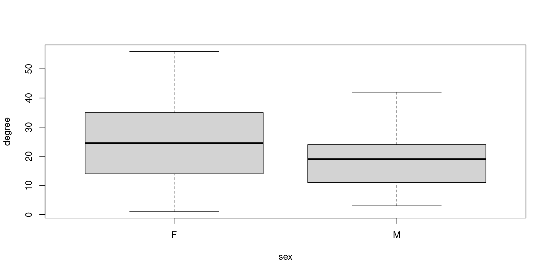
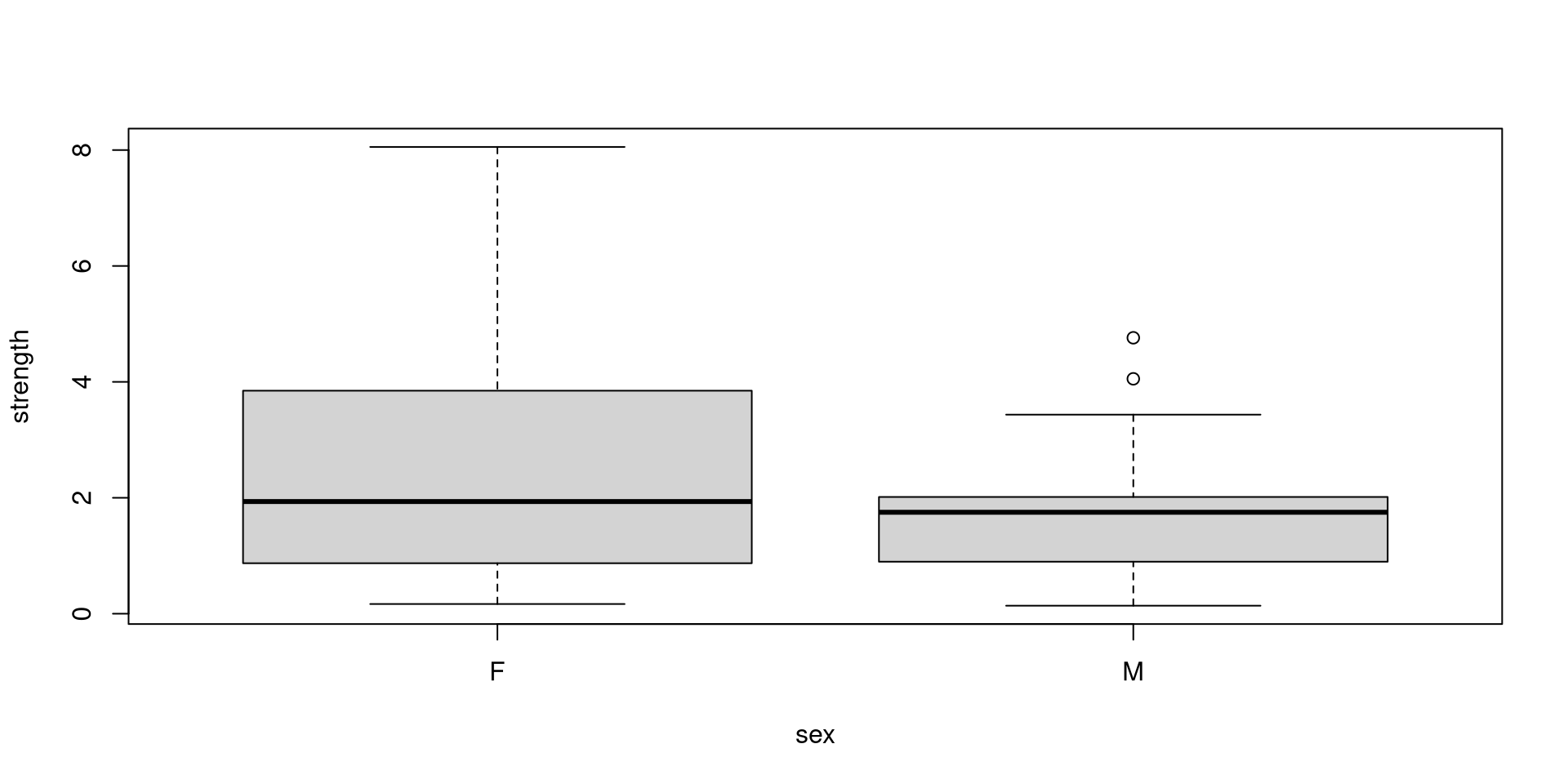
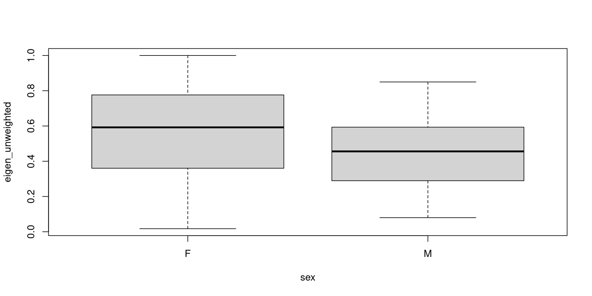
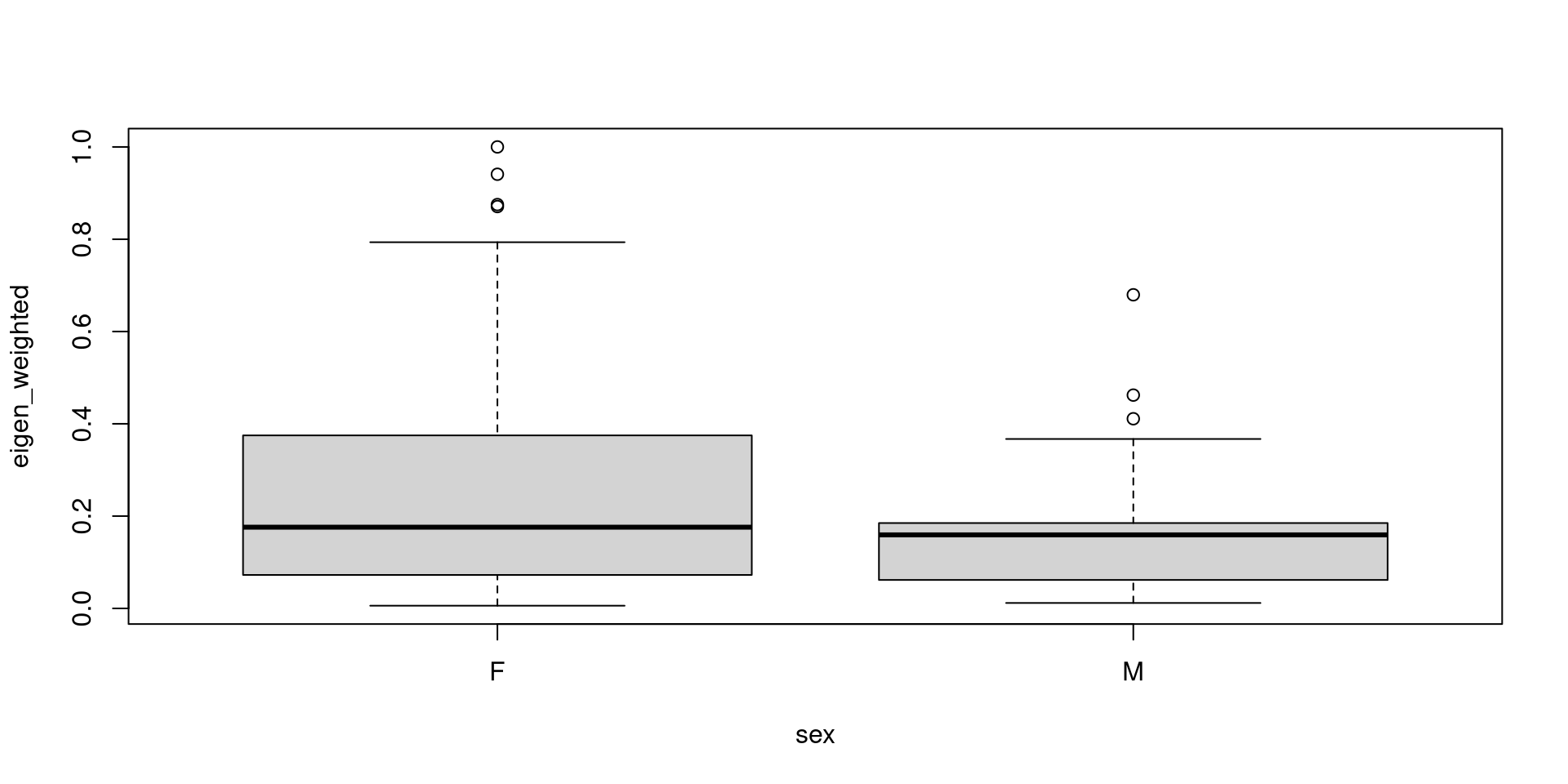
Real Example: Are Male or Female Squirrels more central?
We can plot the results against another vertex attribute. The easiest way is to extract the data from our network using the as_data_frame(network, what="vertices")
Real Example: Are Male or Female Squirrels more central?
We can plot the results against another vertex attribute. The easiest way is to extract the data from our network using the as_data_frame(network, what="vertices")
Measures of Structure
You can also be influential in a network if you can reach everyone easily.
Do you need to have a lot of connections? Not necessarily
Distances
If two nodes are in the same component then there exists at least one path between them.
The path is a set of edges from one node to another that never repeats a node or edge.
The number of edges on the shortest path is called the geodesic distance between those two nodes.
For directed networks the paths are assumed to follow the direction of the edges (but we can drop this if we want to).
Closeness
Closeness is measured by looking at how far a node is from all other nodes. It We start by summing all the distances between the node of interest and all other nodes:
\[ clo_i = \frac{n-1}{\sum_{j} d_{ij}} \]
The closeness of node i (\(clo_i\)) is the number of nodes (\(n\)) minus 1 divided by the sum of the distance between i and every other nodes.
What is the problem here?
Closeness Alternative - Harmonic Centrality
One alternative is to flip this equation around slightly:
In this case, a 1 means that a node is directly connected to every node, a 0 means they are totally isolated.
This is referred to as the Harmonic Centrality
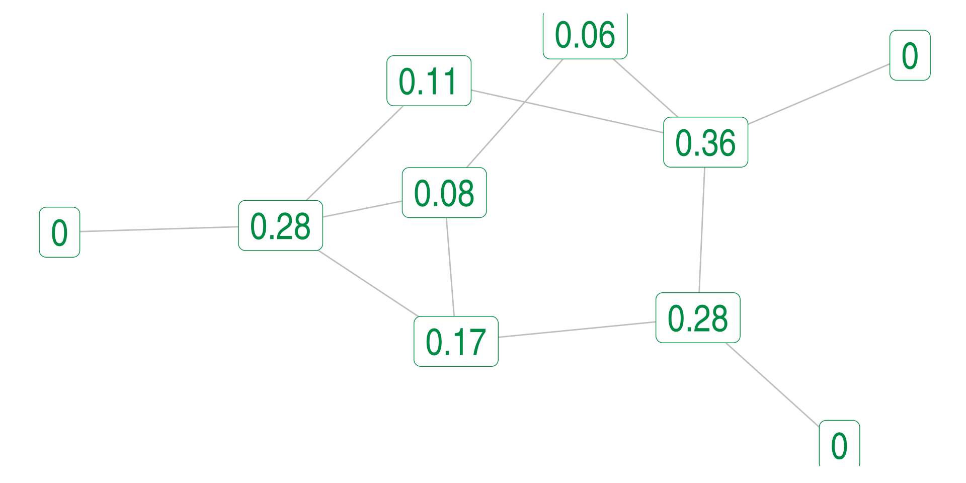
Closeness Example
Harmonic Mean Example
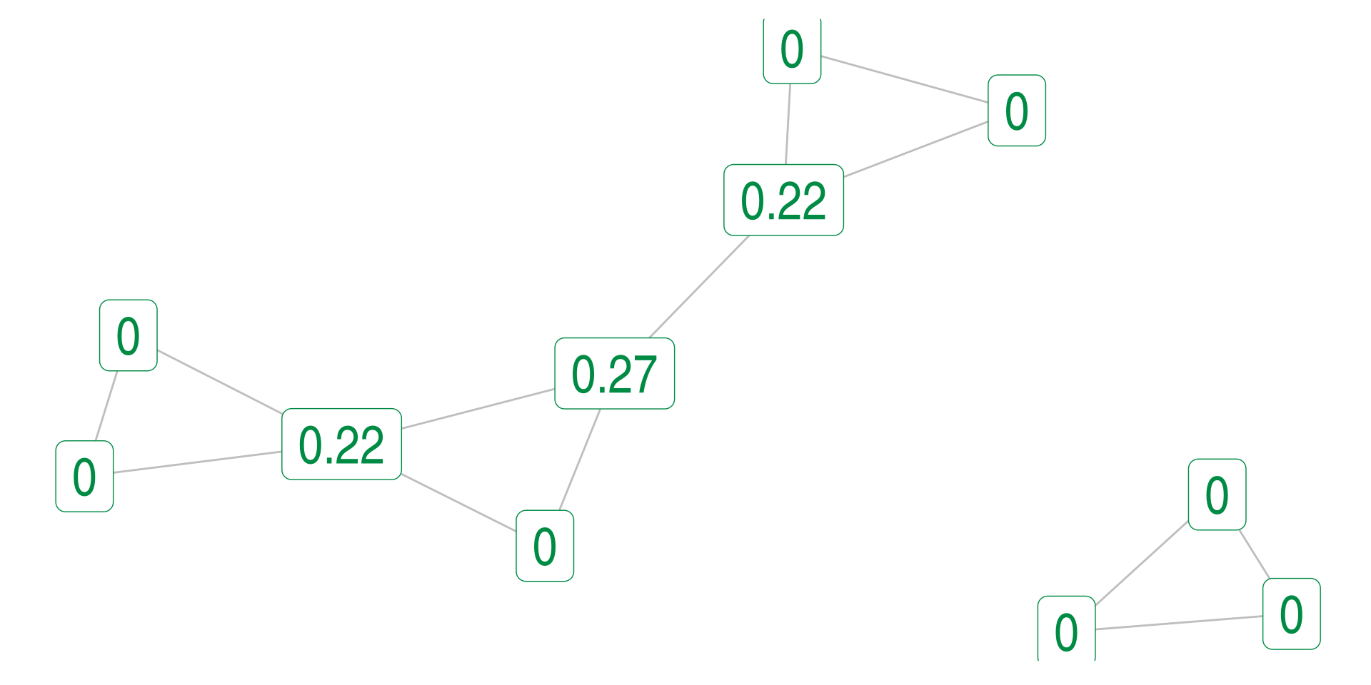
Closeness Example - Disconnected
Note: The igraph implementation only considers reachable nodes.
Harmonic Mean - Disconnected
Betweenness
Betweenness is also about the the idea of geodesic distances.
If a node (j) is on the only geodesic between two other nodes (i) and k) then it is likely that any thing flowing between i and k will pass by k.
But it is possible for multiple geodesic paths to exist between two nodes.
Betweenness
This gives us the formula:
\[ b_j = \sum \frac{g_{ijk}}{g_{ik}} \]
Where \(g_{ijk}\) is the number of geodesic paths between i and k that includes j, while \(g_{ik}\) is the total number of geodesic paths between i and k.
The betweenness score of a node then is the sum of the proportion of geodesics that that node is on between all dyads in a network.
Betweenness Example
Betweenness Example Disconnected
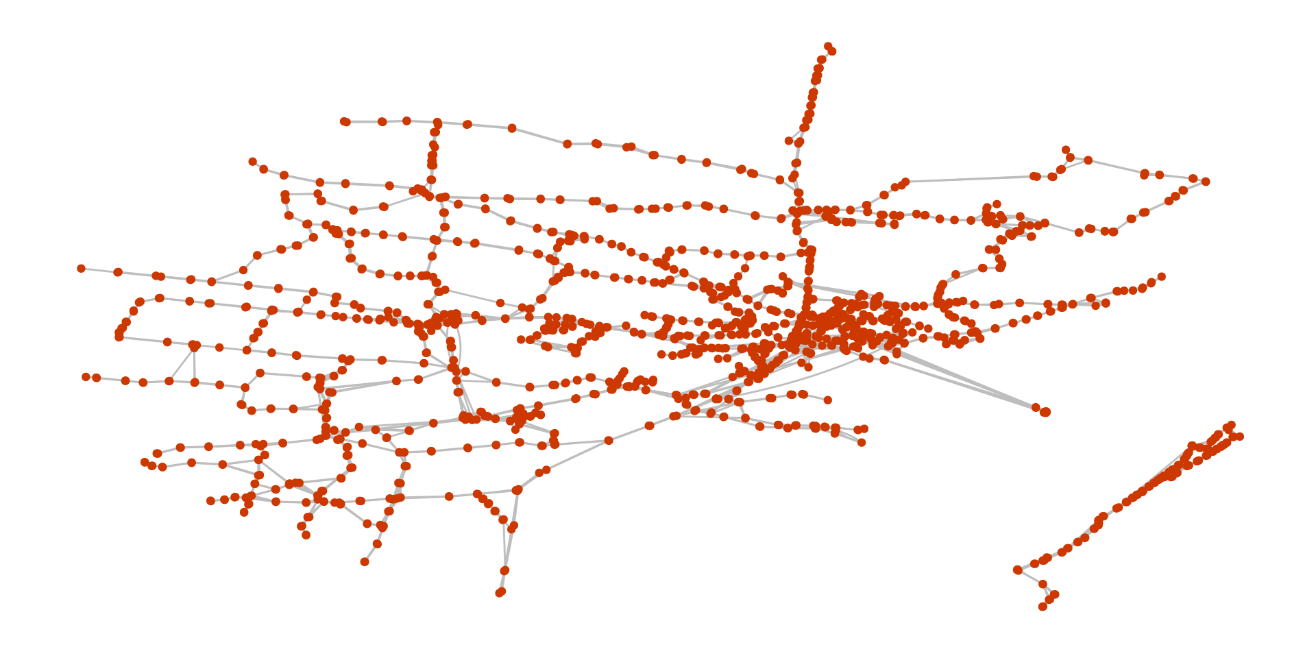
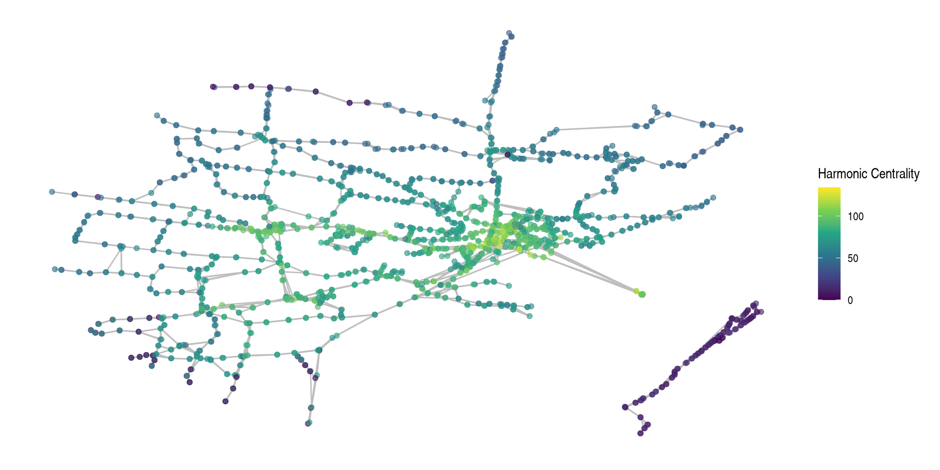
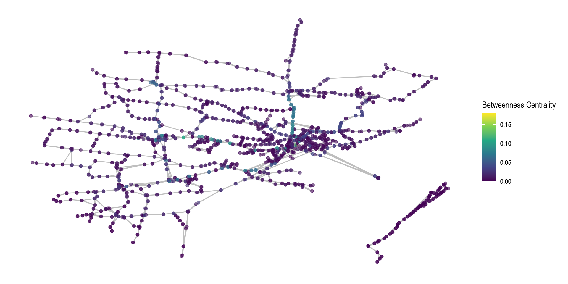
Real Example
Anyone know what this is?
Which Station is Closest?
Which Station is Between Everything?
Directed
When dealing with directed networks there is not much to be done to change the measures.
For *harmonic and closeness we use the directed distance and either calculate the distance to or from a vertex.
For betweenness we don’t have to change anything.
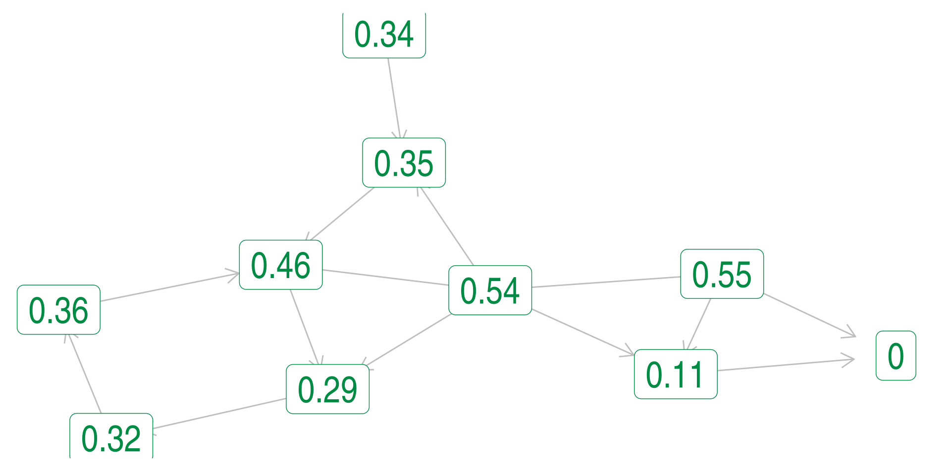
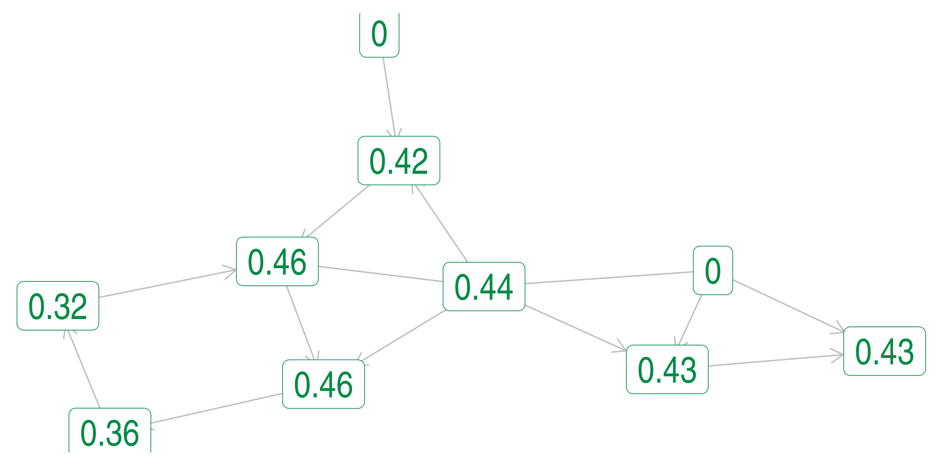
Directed Harmonic Example
Outward
Inward
Weighted
Weighted networks are also relatively easy to accommodate by using the weights in the distance calculation.
There are some ways to do this:
Add the weights along the path as they are (works well if weights represent something like time from node A to B)
Add the inverse of the weights along the path (works well if larger weights mean a closer connection)
Doing this in R
Lets work with a network of the Paris rail system available here.
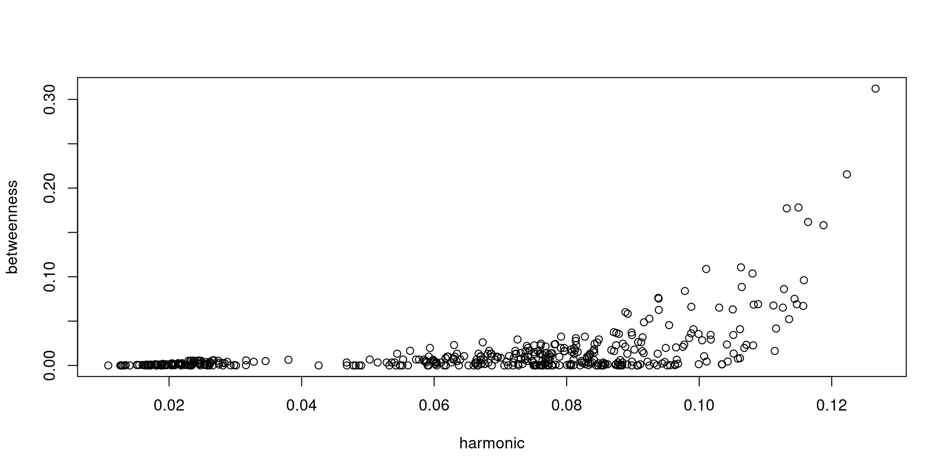
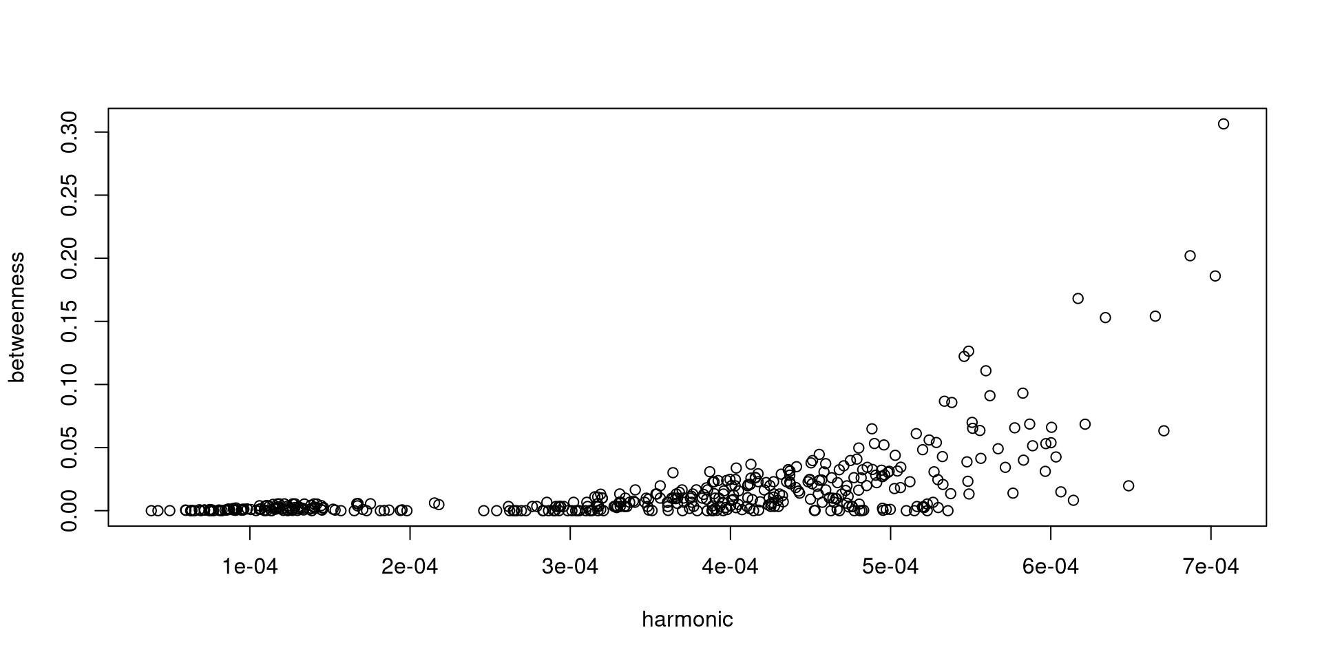
But what if we want to consider, how many trains are moving between these nodes. If we consider the number of trains we wouldn’t want to just add this up.Why?
       lat      lon   between        hc   id     harmonic        station_name
1 48.86182 2.347013 0.3064686 0.1266185 n301 0.0007078619 CHATELET LES HALLES
2 48.85334 2.346035 0.2019850 0.1187620 n302 0.0006869859  ST MICHEL ND RER B
3 48.89219 2.237018 0.1859747 0.1222938 n140 0.0007026697          LA DEFENSE
4 48.88077 2.357115 0.1681275 0.1164376 n300 0.0006170070          PARIS NORD
5 48.87216 2.329927 0.1541205 0.1149822 n370 0.0006652522               AUBER
Using These Measures
Regression Analysis
Measures of centrality are commonly used as DV or IV in regression analysis, but this can be tricky.
Measure of one nodes centrality is dependent on the centrality of other nodes.
If Node A and B have an edge, and I remove that edge both their degrees change.
One approach to this is with Quadratic Assignment Procedure (QAP).