Scaling and Visualization

R
POL 491
Network Analysis

Scaling and Visualization

Doing this in R

There are three main functions we will need for this:

  • mds() from the smacof package.
  • ca() from the ca package.
  • hclust() a base R function (along with cutree() and dist()).

MDS Scaling

The mds() function in smacof lets us estimate multiple types of MDS:

  • mds(distance, type="interval") - Metric MDS
  • mds(distance, type="ordinal") - Non-Metric MDS

In both cases the distance object needs to be a symmetric dissimilarity (distance) matrix. Larger values mean observations are more different from each other.

You select the number of dimensions using ndim=

Recreating a Map from Distances

R has an object UScitiesD that you can call at anytime which shows the distances between several cities.

# UScitiesD #Run this by itself to see
library(smacof)
mds <- mds(UScitiesD, type = "interval")
mds$stress # The stress
[1] 0.001913151
mds$conf # the actual points
                      D1          D2
Atlanta       -0.4543817  0.09024782
Chicago       -0.2415148 -0.21576888
Denver         0.3051669 -0.01607968
Houston       -0.1021788  0.36232737
LosAngeles     0.7612104  0.24459966
Miami         -0.7164226  0.36679903
NewYork       -0.6783018 -0.32755339
SanFrancisco   0.8982951  0.06986850
Seattle        0.8477661 -0.36291042
Washington.DC -0.6196388 -0.21153000

Recreating a Map from Distances

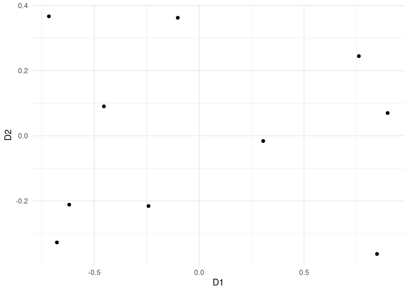
We can plot this with ggplot2

library(ggplot2)

Attaching package: 'ggplot2'
The following object is masked from 'package:e1071':

    element
points <- as.data.frame(mds$conf)
ggplot(points, aes(x = D1, y = D2)) +
  geom_point() +
  theme_minimal()

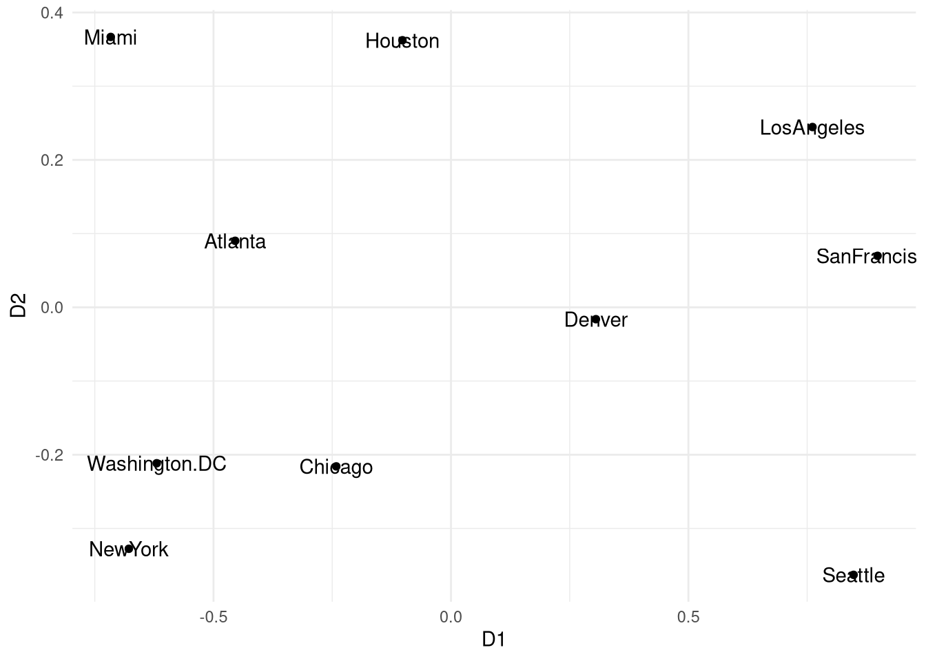
Lets add some labels

points$names <- rownames(points)
ggplot(points, aes(x = D1, y = D2)) +
  geom_point() +
  geom_text(aes(label = names)) +
  theme_minimal()

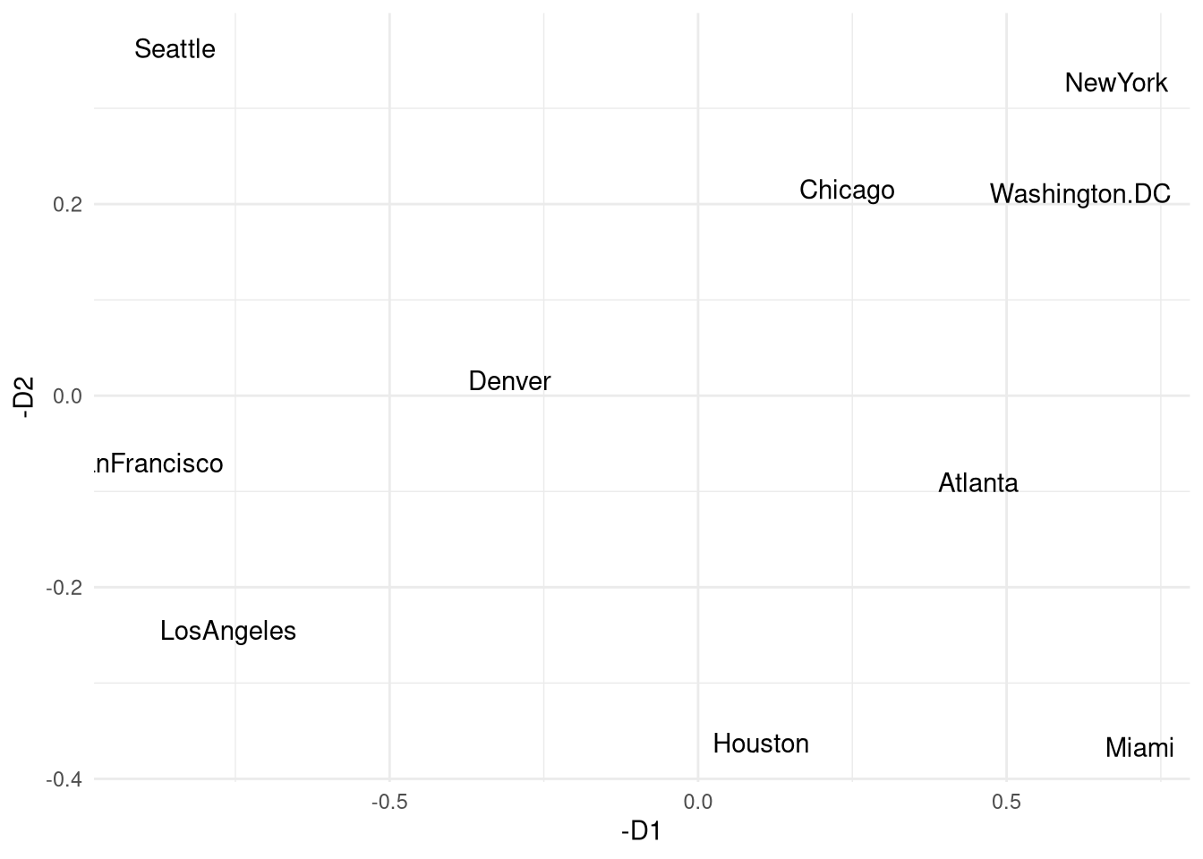
Flip the scales

ggplot(points, aes(x = -D1, y = -D2)) +
  geom_text(aes(label = names)) +
  theme_minimal()

Finding the Number of MDS Dimensions

UN Data

For the next section we are going to use data on UN Votes (this is in an RData format and is already a distance object).

UN_votes <- readRDS(here::here("resources/network_data/distance_1960s.RData"))

out <- mds(UN_votes, ndim = 2, type = "ordinal")
out$stress
[1] 0.1247679

Estimating Many Models

If we want to check different levels of stress we could estimate several models like this:

out_1 <- mds(UN_votes, ndim = 1, type = "ordinal")
out_2 <- mds(UN_votes, ndim = 2, type = "ordinal")
out_3 <- mds(UN_votes, ndim = 3, type = "ordinal")
out_4 <- mds(UN_votes, ndim = 4, type = "ordinal")

This is repetitive, and good code minimizes repetition.

Using a Loop

We can use a for loop to repeat some lines of code multiple times changing things as we do:

Basic idea:

for (ii in 1:5) {
  print(ii)
}
[1] 1
[1] 2
[1] 3
[1] 4
[1] 5

More Complicated Loop

We want to create something to store the results and then store it every time we go through the loop.

out <- numeric(5) ## Vector of length 5
for (ii in 1:5) {
  out[ii] <- ii
}
print(out)
[1] 1 2 3 4 5

Using a Loop to Estimate Models

We want to create something to store the results and then store it every time we go through the loop.

out <- numeric(5) ## Vector of length 5
for (ii in 1:5) {
  tmp <- smacof::mds(UN_votes, ndim = ii, type = "ordinal")
  out[ii] <- tmp$stress
}
print(out)
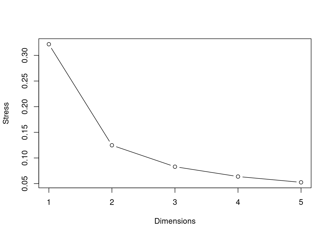
[1] 0.32174980 0.12476788 0.08293623 0.06374924 0.05249708

Scree Plot

I use the basic plot() function to make a scree plot:

plot(x = 1:5, y = out, ylab = "Stress", xlab = "Dimensions", type = "b")

Hierarchical Clustering

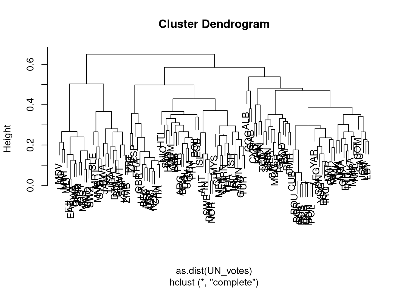
The hclust() function needs a distance object to work. Our UN_votes data already shows “distances” but isn’t a distance object so we use as.dist() to convert it.

hcl <- hclust(as.dist(UN_votes))
plot(hcl) ## creates a dendrogram

Methods of Aggregation

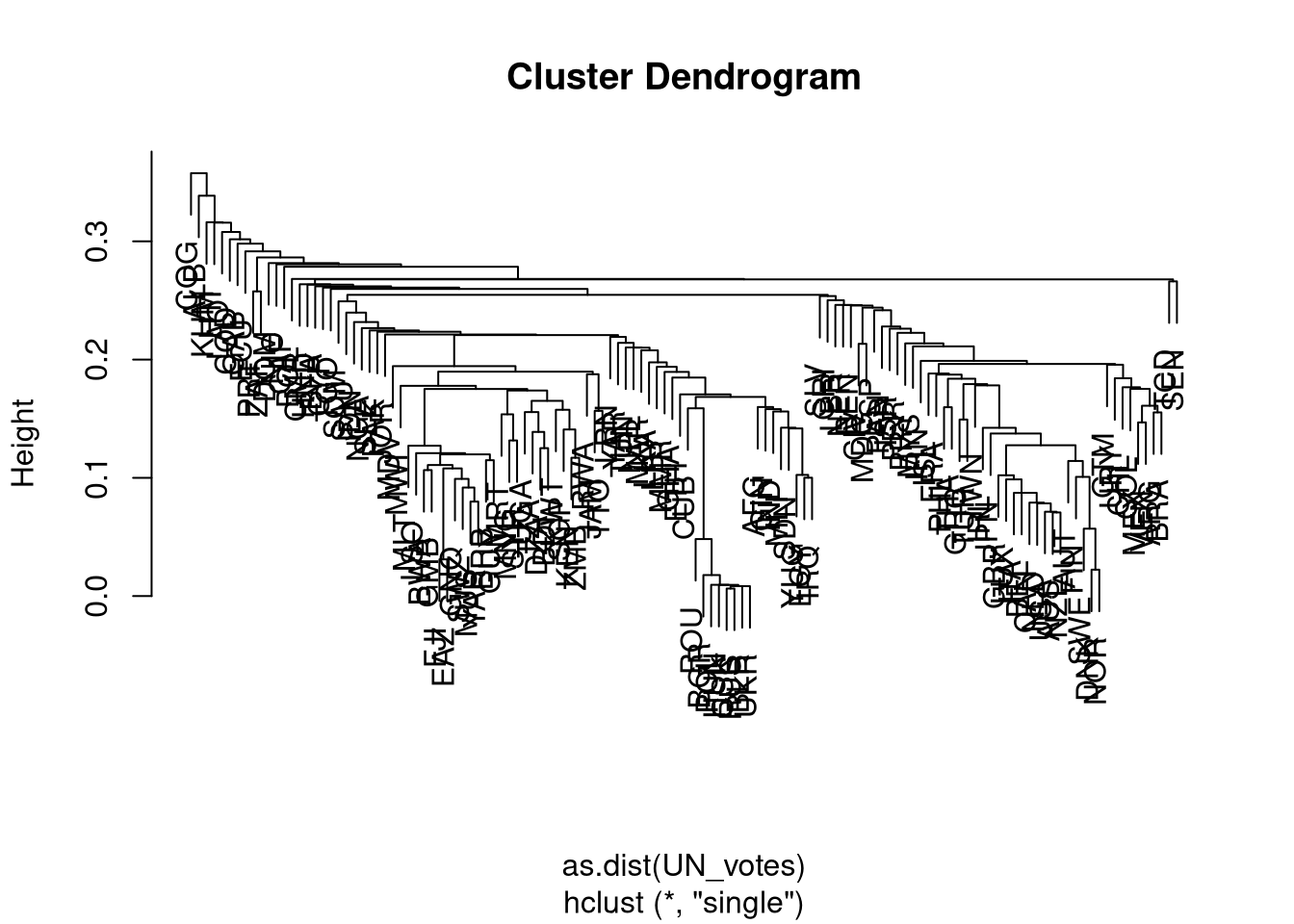
You can change the method with the method= argument (“single”, “complete”, “average”)

hcl <- hclust(as.dist(UN_votes), method = "single")
plot(hcl) ## creates a dendrogram

Creating Groupings

The cutree() function “cuts the tree” to make clusters. Set k= to set the number of groups you want.

groups <- cutree(hcl, k = 4)
groups[1:20]
AFG ALB DZA ARG AUS AUT BRB BLR BEL BEN BOL BWA BRA BGR BFA BDI CIV KHM CMR CAN 
  1   2   1   1   1   1   1   1   1   1   1   1   1   1   1   1   1   3   1   1 

Correspondence Analysis

For correspondence analysis we use the ca() function, as a default it will estimate the largest possible number of dimensions.

The data here shows the number of a majors that graduated from colleges in Ohio in 2024.

mat <- read.csv(
  here::here("resources/network_data/colleges.csv"),
  row.names = 1
)
mat <- as.matrix(mat)
colnames(mat) <- gsub("\\.", " ", colnames(mat))

library(ca)

ca_out <- ca(mat)

Correspondence Analysis - Dimensions

If you call summary() on your ca() object then the top of it will show you how much variance each dimension captures.

summary(ca_out)

Principal inertias (eigenvalues):

 dim    value      %   cum%   scree plot               
 1      0.117421  23.5  23.5  ******                   
 2      0.080262  16.0  39.5  ****                     
 3      0.066208  13.2  52.8  ***                      
 4      0.046961   9.4  62.2  **                       
 5      0.036803   7.4  69.5  **                       
 6      0.034299   6.9  76.4  **                       
 7      0.024345   4.9  81.2  *                        
 8      0.024097   4.8  86.1  *                        
 9      0.017228   3.4  89.5  *                        
 10     0.013851   2.8  92.3  *                        
 11     0.008533   1.7  94.0                           
 12     0.008314   1.7  95.6                           
 13     0.006164   1.2  96.9                           
 14     0.004779   1.0  97.8                           
 15     0.003641   0.7  98.6                           
 16     0.002463   0.5  99.1                           
 17     0.001591   0.3  99.4                           
 18     0.001178   0.2  99.6                           
 19     0.000675   0.1  99.7                           
 20     0.000543   0.1  99.9                           
 21     0.000357   0.1  99.9                           
 22     0.000193   0.0 100.0                           
 23     0.000174   0.0 100.0                           
 24     2e-05000   0.0 100.0                           
        -------- -----                                 
 Total: 0.500099 100.0                                 


Rows:
     name   mass  qlt  inr     k=1 cor ctr     k=2 cor ctr  
1  | Edct |   61  652   85 |  -621 549 200 |  -268 102  54 |
2  | AECG |    4  697   42 |  1174 234  42 | -1650 463 121 |
3  | BlBS |   65  570   25 |   319 528  57 |    90  42   7 |
4  | BMMR |  213  350   57 |  -185 257  62 |   112  93  33 |
5  | ELLL |   16  593   14 |   210  98   6 |  -471 495  43 |
6  | Hstr |    9  682   11 |   429 329  15 |  -444 353  23 |
7  | LASG |    9   72   62 |  -479  68  18 |  -117   4   2 |
8  | MlIS |   19   15   34 |  -111  13   2 |   -35   1   0 |
9  | NtRC |   11  394   19 |   463 264  21 |  -324 130  15 |
10 | PhRS |    4  166   31 |   515  67   9 |  -630 100  19 |
11 | Psyc |   57  311    9 |   138 250   9 |   -68  61   3 |
12 | SclS |   55  404   36 |   360 403  61 |   -24   2   0 |
13 | VsPA |   45  735   77 |   254  76  25 |  -747 658 315 |
14 | FCSH |   10  109   24 |   327  85   9 |   171  23   4 |
15 | HPRP |  132   42   83 |   -15   1   0 |   113  41  21 |
16 | PASS |   15   54   17 |     2   0   0 |   173  54   6 |
17 | CJRP |   47   21   21 |    67  21   2 |     7   0   0 |
18 | CmIS |   36   16   37 |    -6   0   0 |    92  16   4 |
19 | FLLL |    9  619   10 |   510 497  21 |  -254 123   8 |
20 | HSLE |   22  772   98 | -1318 763 320 |  -137   8   5 |
21 | MthS |   12  471   11 |   454 456  22 |   -82  15   1 |
22 | PRLF |   26  175   34 |  -180  49   7 |  -287 126  26 |
23 | PhyS |   14  436   11 |   350 316  14 |  -215 119   8 |
24 | Engn |   92  672   85 |   258 144  52 |   494 527 281 |
25 | ArRS |    7    4   16 |     3   0   0 |   -69   4   0 |
26 | EETT |   10  121   52 |  -574 121  27 |    -7   0   0 |

Columns:
     name   mass  qlt  inr     k=1 cor ctr     k=2 cor ctr  
1  | AshU |    9  230   11 |  -344 204   9 |  -124  26   2 |
2  | BlWU |   12  527   15 |   -10   0   0 |  -568 527  48 |
3  | BGSU |   50  486   57 |  -391 269  65 |  -351 217  77 |
4  | CWRU |   27  414   53 |   551 314  71 |   310 100  33 |
5  | CdrU |   15   45    7 |   -18   1   0 |   -98  44   2 |
6  | CnSU |   18  711  123 | -1507 683 357 |  -303  28  21 |
7  | ClSU |   38   89   17 |   139  89   6 |    10   0   0 |
8  | DnsU |   11  519   31 |   584 253  33 |  -600 266  51 |
9  | FrUS |    9   53   33 |   165  14   2 |  -270  38   8 |
10 | FrnU |   28  307   80 |  -639 285  97 |   177  22  11 |
11 | JhCU |   11   21   18 |     4   0   0 |  -134  21   2 |
12 | KSUK |   78  472   32 |  -144 102  14 |  -274 370  73 |
13 | MmUO |   71   26   40 |    58  12   2 |   -62  14   3 |
14 | ObrC |   15  851  117 |  1039 274 136 | -1509 577 420 |
15 | OhNU |    9  136    6 |    19   1   0 |   221 135   5 |
16 | OSUM |  204  616   81 |   287 414 143 |   201 203 103 |
17 | OUMC |   80    1   66 |    23   1   0 |     8   0   0 |
18 | OttU |    9  418   12 |   318 148   8 |  -428 269  20 |
19 | UAMC |   35  267   28 |  -218 119  14 |   244 148  26 |
20 | UCMC |  114  120   36 |   -19   2   0 |   136 117  26 |
21 | UnfD |   36  221   17 |  -127  70   5 |   187 151  16 |
22 | UnfT |   43  219   37 |   -93  20   3 |   293 199  46 |
23 | WSUM |   24   16    9 |    11   1   0 |   -55  15   1 |
24 | XvrU |   23   64   24 |  -141  39   4 |  -114  25   4 |
25 | YnSU |   29  135   52 |  -338 130  29 |   -64   5   1 |

Correspondence Analysis - Plotting One Set

If we want to extract the scales we use cacoord() which has a variety of options under type=. What we want is either "rowprincipal" or "colprincpal"

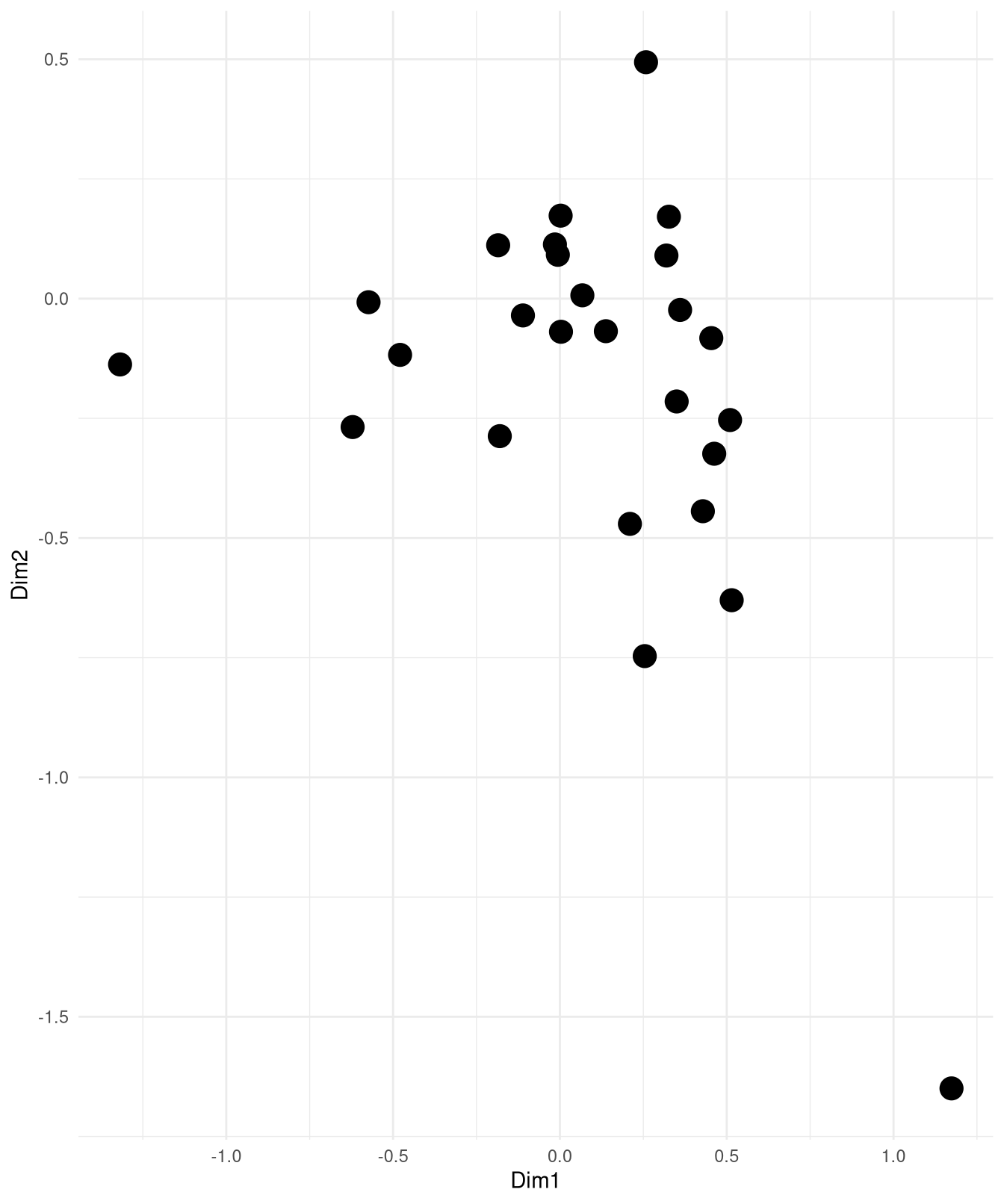
majors_principal <- cacoord(ca_out, type = "rowprincipal")
ggplot(majors_principal$rows, aes(x = Dim1, y = Dim2)) +
  geom_point(size = 5) +
  theme_minimal()

Basic scatter plot showing dots on a Dim 1 and Dim 2 axis. The points are the majors.

Correspondence Analysis - Plotting Both

It will return an object with both $rows and $columns. If this is row principals then the rows are in principal components and the columns are standard components.
majors <- as.data.frame(majors_principal$rows)
majors$Type <- "Majors"
majors$Name <- rownames(majors)
schools <- as.data.frame(majors_principal$columns)
schools$Type <- "School"
schools$Name <- rownames(schools)

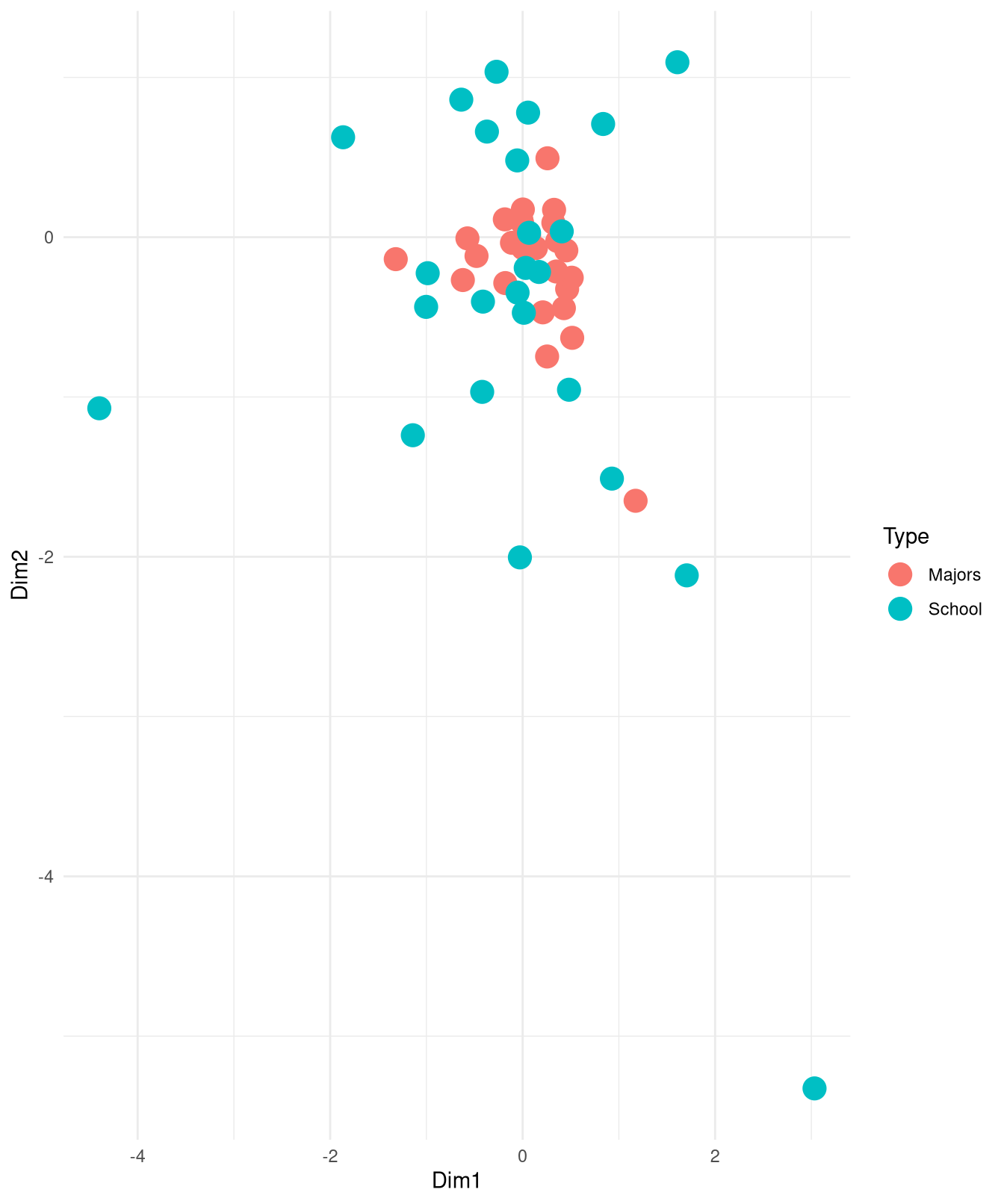
all <- rbind(majors, schools)

ggplot(all, aes(x = Dim1, y = Dim2, color = Type)) +
  geom_point(size = 5) +
  theme_minimal()

Basic scatter plot showing dots on a Dim 1 and Dim 2 axis. The majors and schools are colored differently here.

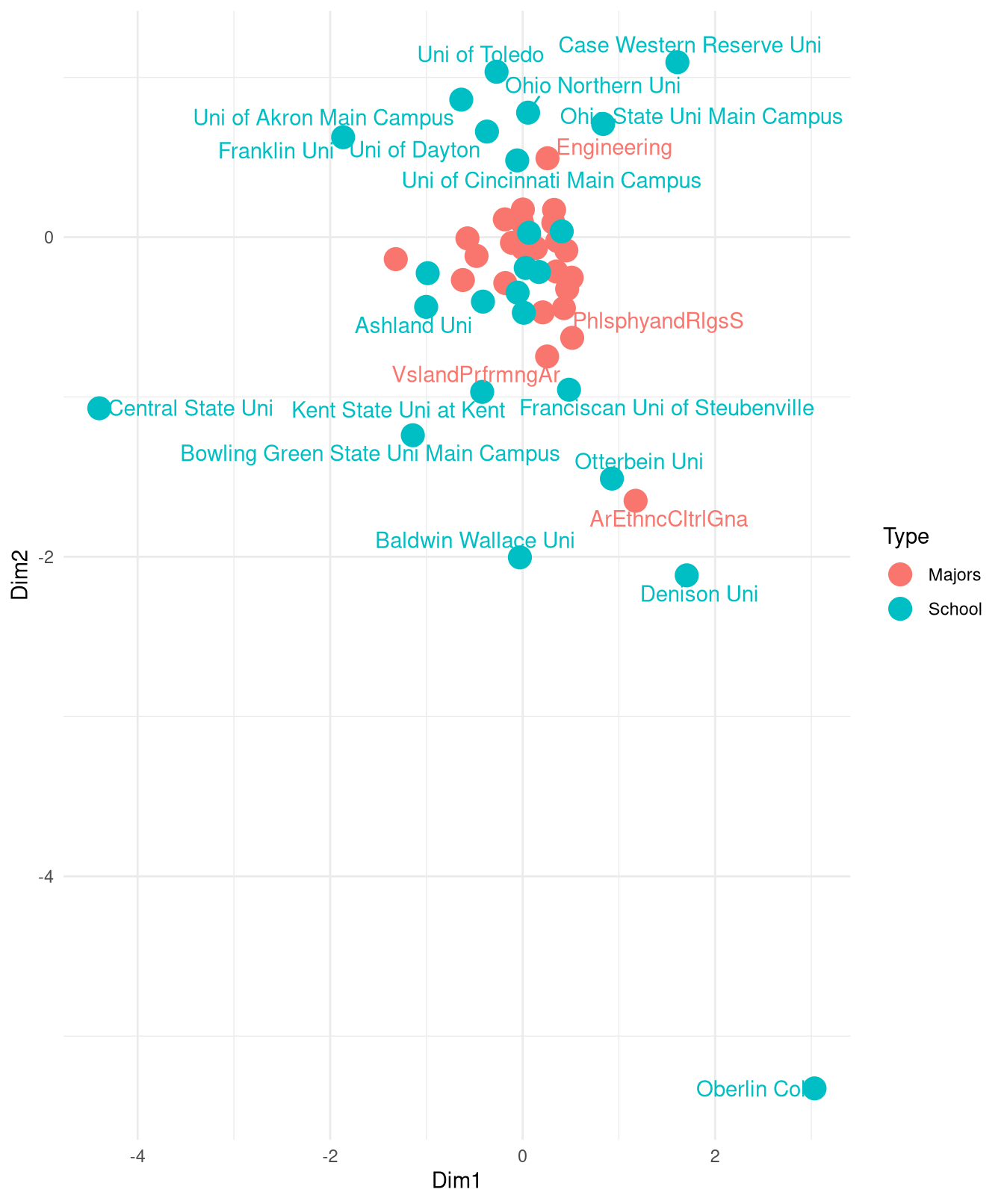
To add labels you can use geom_repel_text() from the ggrepel library.

library(ggrepel)

ggplot(all, aes(x = Dim1, y = Dim2, color = Type)) +
  geom_point(size = 5) +
  theme_minimal() +
  geom_text_repel(aes(label = Name))