Using igraph
R
POL 491
Network Analysis
Networks are complicated objects compared to more standard types of data that you are probably used to. Most datasets are a simple rectangle with \(n\) rows and \(p\) columns. Networks though can not easily fit into this format. Although there are \(n\) nodes (rows), we need to have information on how those \(n\) nodes are connected to each other and we also want to be able to store information about the nodes (usually our columns \(p\)) and sometimes even information about our edges.
This section walks through the basics of network objects in R, focusing on how igraph handles network objects. igraph has its own native way of storing networks (which is what I call the network object). Some of this will look like how you manipulate data frames in R, some of it will be entirely unique. Before using igraph though I want to first show how a basic adjacency matrix can be created in R and then convert that to a network object (you won’t normally do this while loading data, but it is a good starting point).
Simple Adjacency Matrices
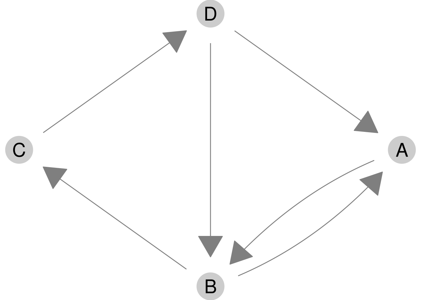
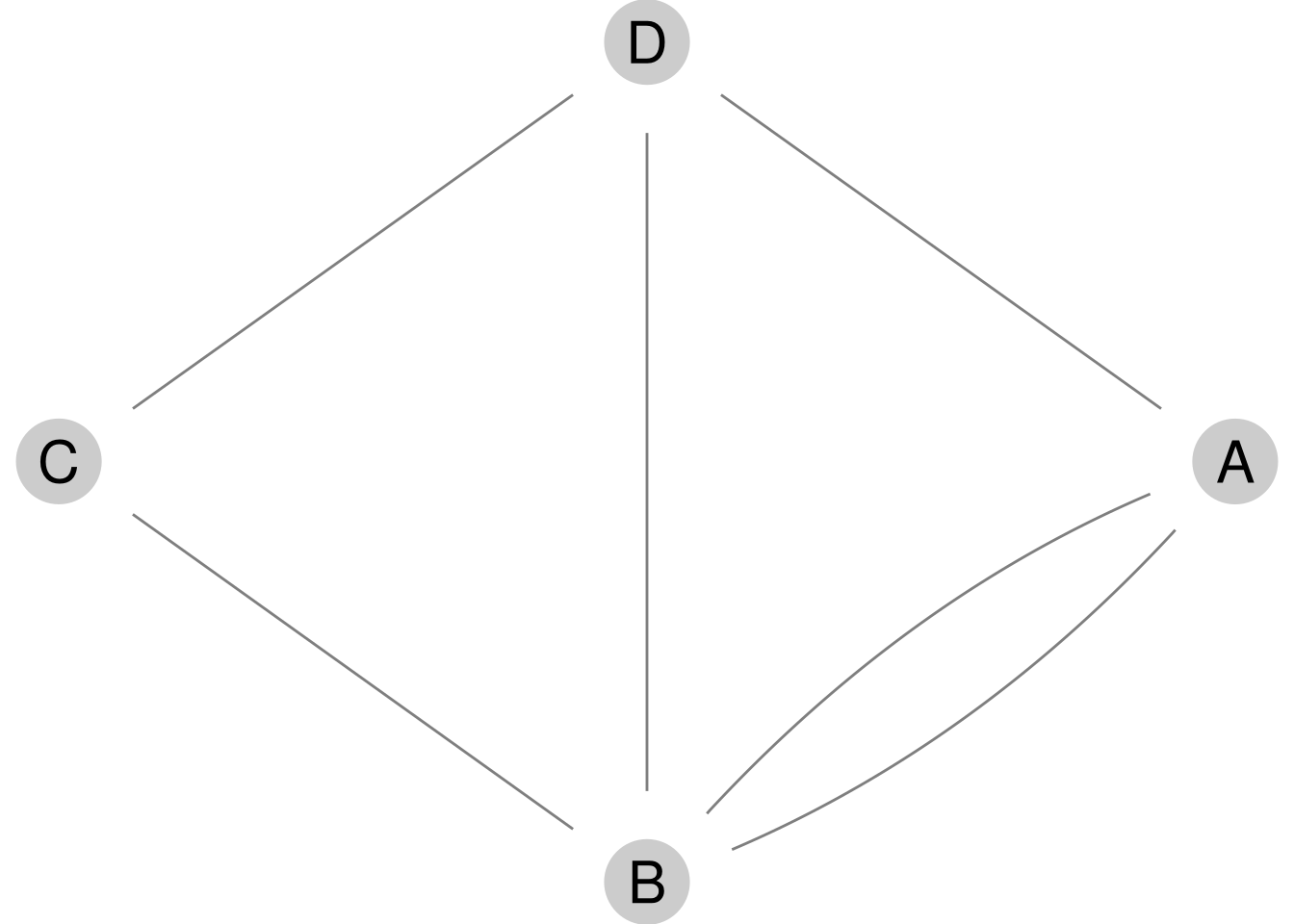
Remember, one of the basic formats to capture the structure of a network is an adjacency matrix. This is a square matrix with \(n\) rows and \(n\) columns where \(n\) is the number of nodes. In Equation 1 there is an adjacency matrix with four nodes. Letting the rows and columns be A, B, C, and D, we can see that A has an edge to B, B has edges to A and C, etc. The full network visualization is shown in Figure 1.
Although I have not explicitly written that A is a directed network, you should be able to tell. Undirected adjacency matrices ought to be symmetric1 meaning that the values are mirrored across the diagonal. Since this is not the case here, A is a directed network.
\[ A=\begin{pmatrix} 0 & 1 & 0 & 0 \\ 1 & 0 & 1 & 0 \\ 0 & 0 & 0 & 1 \\ 1 & 1 & 0 & 0 \\ \end{pmatrix} \tag{1}\]
We can recreate this matrix in R using the matrix() function. The matrix function takes a vector and fils in a matrix column by column. I find it useful to set byrow=TRUE to fill in the matrix row by row instead as then I can write out the matrix I want as a vector using linebreaks. We can also set the number of rows and columns using nrow= and ncol=.2
# fmt: skip
mat <- matrix(
  c(0, 1, 0, 0,
    1, 0, 1, 0,
    0, 0, 0, 0,
    1, 1, 1, 0),
  nrow = 4,
  ncol = 4,
  byrow = TRUE
)
mat
[,1] [,2] [,3] [,4]
[1,] 0 1 0 0
[2,] 1 0 1 0
[3,] 0 0 0 0
[4,] 1 1 1 0Although this is not entirely necessary, we can set the row names and columns
rownames(mat) <- LETTERS[1:nrow(mat)]
colnames(mat) <- rownames(mat)
mat
A B C D
A 0 1 0 0
B 1 0 1 0
C 0 0 0 0
D 1 1 1 0igraph Objects
Although we can do a lot with basic matrices, what we really want to create is an object that is recognized as a network. This will let us interface with other R functions that expect a network object, and allow us to store information about the nodes and edges.
The igraph package has a suite of functions that start with graph_from_ which are used to create network objects from a variety of data formats. For our adjacency matrix we will use the aptly named graph_from_adjacency_matrix() function.
mode="directed"directed network."undirected"undirected, using upper triangle to make. Deprecated"max"undirected, using max of upper and lower triangle."min"undirected, using min of upper and lower triangle."upper"undirected, using upper triangle."lower"undirected, using lower triangle."plus"undirected, using sum of upper and lower triangle.
weighted=NULL(default) the numbers in matrix give the number of edges betweenTRUEcreates edge weights using the values in the matrix as the “weight” attribute.- Any other character will be used as the name of the edge attributes to store the values in the matrix.
diag=whether to include the diagonal elements of the matrix (meaning self-loops). Defaults toFALSE.add.colnames=NULL(default) use column names as the vertex names.NAignore the column names.
The below code converts our basic adjacency matrix into an igraph object. If you call the object (the second line) you can see that now different information is displayed. In particular it provides a list of attributes (in this case the only one is “name”), and then the edges of the network. For larger networks it will show only a limited number of edges. Since the network is directed, the edges show that direction.
library(igraph)
net <- graph_from_adjacency_matrix(mat, mode = "directed")
net
IGRAPH 4ab6239 DN-- 4 6 --
+ attr: name (v/c)
+ edges from 4ab6239 (vertex names):
[1] A->B B->A B->C D->A D->B D->CBasic Commands
We will learn how to do a lot with network objects but for now we can look at some very simple functions.
ecount()Returns the number of edges in a network.vcount()Returns the number of vertices in a network.degree()Returns the degree of each node (for directed networks usemode=to select either"out","in", or"total"degrees).count_components()Returns the number of components in the network (if directed setmode=to either"strong"or"weak"to determine what type of components).
ecount(net)[1] 6vcount(net)[1] 4degree(net, mode = "out")A B C D
1 2 0 3 degree(net, mode = "in")A B C D
2 2 2 0 count_components(net, mode = "weak")[1] 1count_components(net, mode = "strong")[1] 3Converting to Undirected
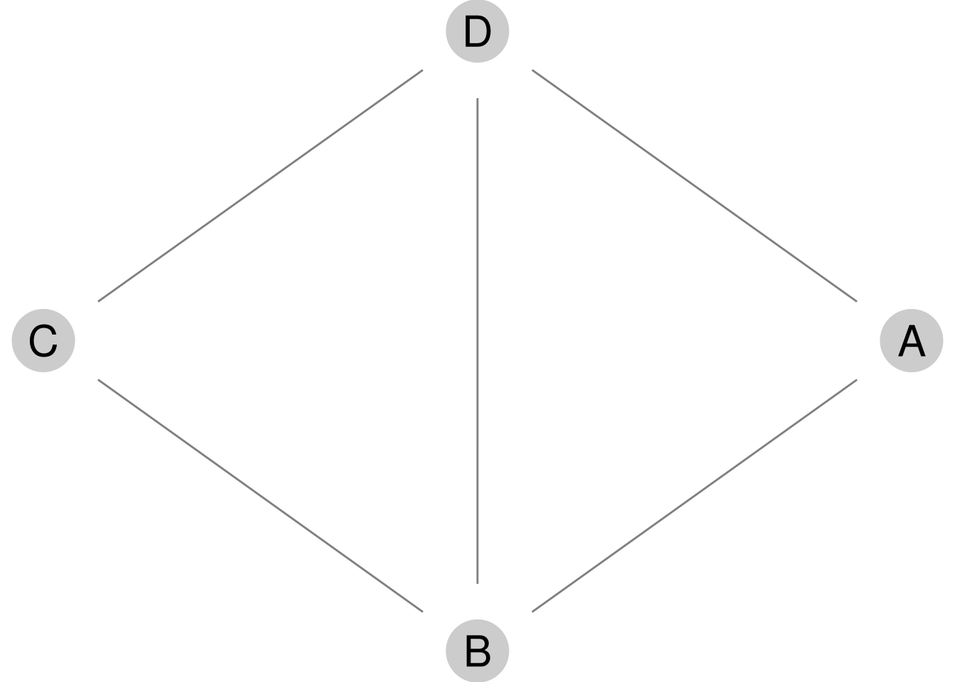
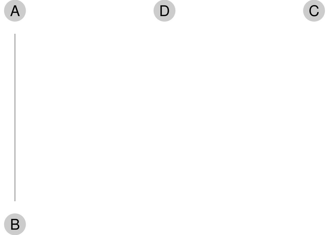
It is not uncommon in network research to convert a directed network to an undirected network. This can be done for a lot of reasons, but often it is because some network methods work better on undirected networks. In some cases this is called symmetrizing. To do this in igraph we use as_undirected() but we have to decide in what context an undirected edge should exist. Should we only create an undirected edge when there are edges in both directions between nodes? Where there is only one?
mode= again controls when an edge is created. The options are:
"collapse"- Creates 1 undirected edge when there is at least one edge between two nodes (if there is more than 1 then 1 will only be created)."mutual"- Creates 1 undirected edge only when there are edges from each node to the other (so two edges needed)."each"- Creates 1 undirected edge for each each directed edge and so allows multiple edges (least common way to symmetrize)
collapse_net <- as_undirected(net, mode = "collapse")
collapse_net
IGRAPH fc61053 UN-- 4 5 --
+ attr: name (v/c)
+ edges from fc61053 (vertex names):
[1] A--B B--C A--D B--D C--Dmutual_net <- as_undirected(net, mode = "mutual")
mutual_netIGRAPH 68f60ba UN-- 4 1 --
+ attr: name (v/c)
+ edge from 68f60ba (vertex names):
[1] A--Beach_net <- as_undirected(net, mode = "each")
each_netIGRAPH d98e499 UN-- 4 6 --
+ attr: name (v/c)
+ edges from d98e499 (vertex names):
[1] A--B A--B B--C A--D B--D C--D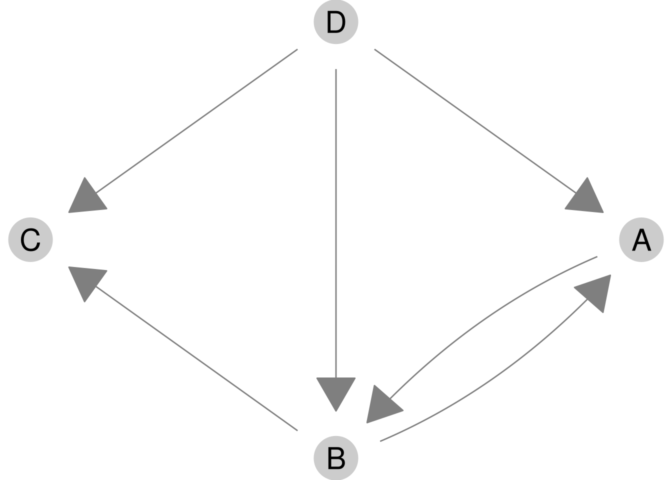
Loading Adjacency Matrix from CSV
Lets load some more interesting data. We need to read in a csv (creating a data frame) of an adjacency csv. Because we know we will make this into an adjacency matrix we set row.names=1 to convert the first column of the csv into row names.
The data is here and is an adjacency matrix based on interactions in the first epsiode of Amazon Prime’s Wheel of Time.
net_mat <- read.csv(
  here::here("resources/network_data/wheel_of_time_ep1.csv"),
  row.names = 1
)
# setting row.names=1, turns the first column into rownames
net_mat[1:5, 1:5] # look at first 5 rows and cols
Moraine Lan Marin Nynavene Rand
Moraine 0 4 1 1 1
Lan 4 0 0 1 0
Marin 1 0 0 1 1
Nynavene 1 1 0 0 1
Rand 1 0 0 0 0Converting to igraph object
We again use graph_from_adjacency_matrix to convert to an igraph object, but first put net_mat into as.matrix(). Why do we set weighted=TRUE?
library(igraph)
net <- graph_from_adjacency_matrix(
  as.matrix(net_mat),
  mode = "directed",
  weighted = TRUE
)
Converting Back to Adjacency Matrix
If we ever want to go back to the adjacency matrix we can:
mat <- as.matrix(net)
mat[1:5, 1:5]
5 x 5 sparse Matrix of class "dgCMatrix"
Moraine Lan Marin Nynavene Rand
Moraine . 1 1 1 1
Lan 1 . . 1 .
Marin 1 . . 1 1
Nynavene 1 1 . . 1
Rand 1 . . . .Another Way to Access the Adj Matrix
The iGraph object actually has the adjacency matrix always there
net[1:5, 1:5]5 x 5 sparse Matrix of class "dgCMatrix"
Moraine Lan Marin Nynavene Rand
Moraine . 4 1 1 1
Lan 4 . . 1 .
Marin 1 . . 1 1
Nynavene 1 1 . . 1
Rand 1 . . . .Making it Undirected (Symmetrizing)
We can also create an undirected network out of a directed network using as.undirected(). The way it creates these depends on mode=.
und_net <- as.undirected(net, mode = "mutual")Warning: `as.undirected()` was deprecated in igraph 2.1.0.
ℹ Please use `as_undirected()` instead.## Undirected edge exists only if both have an edge
as.matrix(und_net)[1:5, 1:5]5 x 5 sparse Matrix of class "dgCMatrix"
Moraine Lan Marin Nynavene Rand
Moraine . 1 1 1 1
Lan 1 . . 1 .
Marin 1 . . . .
Nynavene 1 1 . . .
Rand 1 . . . .Switching it to mode="collapse"
und_net <- as.undirected(net, mode = "collapse")
## Undirected edge exists if either have an edge
as.matrix(und_net)[1:5, 1:5]
5 x 5 sparse Matrix of class "dgCMatrix"
Moraine Lan Marin Nynavene Rand
Moraine . 1 1 1 1
Lan 1 . . 1 .
Marin 1 . . 1 1
Nynavene 1 1 1 . 1
Rand 1 . 1 1 .Access Vertices and Edges
We use the V() and E() functions to access the vertices or edges of our network (note the capitalization)
V(net)+ 22/22 vertices, named, from af397bc:
[1] Moraine Lan Marin Nynavene Rand
[6] Mat Perrin Egwene False.Dragon Eladia
[11] Dying.Man Tam Laila Tom Brandelwyn
[16] Cabin.Trolloc Danya Matt.s.Mom Matt.s.Sisters Padan.Fain
[21] Town.Trolloc Daise E(net)+ 63/63 edges from af397bc (vertex names):
[1] Moraine ->Lan Moraine ->Marin Moraine ->Nynavene
[4] Moraine ->Rand Moraine ->Mat Moraine ->Perrin
[7] Moraine ->Egwene Lan ->Moraine Lan ->Nynavene
[10] Marin ->Moraine Marin ->Nynavene Marin ->Rand
[13] Marin ->Egwene Nynavene->Moraine Nynavene->Lan
[16] Nynavene->Rand Nynavene->Perrin Nynavene->Egwene
[19] Nynavene->Dying.Man Rand ->Moraine Rand ->Mat
[22] Rand ->Perrin Rand ->Egwene Rand ->Tam
[25] Mat ->Moraine Mat ->Rand Mat ->Perrin
[28] Mat ->Danya Mat ->Matt.s.Mom Mat ->Matt.s.Sisters
+ ... omitted several edgesVertex and Edge Attributes
We can have attributes at three different levels of the network: whole network, vertex, and edges. We can get the full list of the different attributes using *_attr_names() functions:
vertex_attr_names(net)[1] "name"edge_attr_names(net)[1] "weight"graph_attr_names(net)character(0)Accessing an Attribute
There are several weights to access a vertex or edge attribute, but the easiest one is to something like: V(net)$attr where attr is the name of the attribute. You can do this with E() as well
V(net)$name [1] "Moraine" "Lan" "Marin" "Nynavene"
[5] "Rand" "Mat" "Perrin" "Egwene"
[9] "False.Dragon" "Eladia" "Dying.Man" "Tam"
[13] "Laila" "Tom" "Brandelwyn" "Cabin.Trolloc"
[17] "Danya" "Matt.s.Mom" "Matt.s.Sisters" "Padan.Fain"
[21] "Town.Trolloc" "Daise" E(net)$weight [1] 4 1 1 1 1 1 1 4 1 1 1 1 2 1 1 1 1 3 1 1 3 4 4 3 1 3 4 1 2 2 1 1 3 3 4 1 1 4
[39] 4 1 1 1 1 1 1 1 1 3 1 1 1 1 1 1 1 2 1 2 1 2 1 1 1Setting Attributes/Modifying Networks
You modify attributes in a way similar to how dataframes are modified in R: E(net)$attr <- "Good"
V(net)$type <- "Character"
V(net)$type
[1] "Character" "Character" "Character" "Character" "Character" "Character"
[7] "Character" "Character" "Character" "Character" "Character" "Character"
[13] "Character" "Character" "Character" "Character" "Character" "Character"
[19] "Character" "Character" "Character" "Character"Indexing Vertices and Edges
Each vertex and edge can be indexed using [ ]. For example V(net)[2] will return the second vertex
V(net)[2]+ 1/22 vertex, named, from af397bc:
[1] LanE(net)[2]+ 1/63 edge from af397bc (vertex names):
[1] Moraine->MarinModifying Attributes
We can also use the indexing to modify the attributes:
V(net)$name[9] ## Missing a space[1] "False.Dragon"V(net)$name[9] <- "False Dragon"
V(net)$name ## Fixed [1] "Moraine" "Lan" "Marin" "Nynavene"
[5] "Rand" "Mat" "Perrin" "Egwene"
[9] "False Dragon" "Eladia" "Dying.Man" "Tam"
[13] "Laila" "Tom" "Brandelwyn" "Cabin.Trolloc"
[17] "Danya" "Matt.s.Mom" "Matt.s.Sisters" "Padan.Fain"
[21] "Town.Trolloc" "Daise" Handling Edges
Dealing with edges can be a bit more confusing, they also have IDs. The best way to identify them is to identify them by what vertex they are incident to.
Identifying Edge IDs
get.edge.ids() will give you the edges from one vertex to another (given using the vp= argument)
V(net)[5] # Rand+ 1/22 vertex, named, from af397bc:
[1] RandV(net)[6] # Mat+ 1/22 vertex, named, from af397bc:
[1] Matedid <- get.edge.ids(net, vp = cbind(V(net)[5], V(net)[6]))Warning: `get.edge.ids()` was deprecated in igraph 2.1.0.
ℹ Please use `get_edge_ids()` instead.edid[1] 21E(net)[edid]+ 1/63 edge from af397bc (vertex names):
[1] Rand->MatGetting all Incident Edges
incident() is used to get all edges that are incident to a vertex. You can set mode= to decide what to do with directed edges.
incident(net, V(net)[5], mode = "in")+ 7/63 edges from af397bc (vertex names):
[1] Moraine ->Rand Marin ->Rand Nynavene->Rand Mat ->Rand Perrin ->Rand
[6] Egwene ->Rand Tam ->Randincident(net, V(net)[5], mode = "out")+ 5/63 edges from af397bc (vertex names):
[1] Rand->Moraine Rand->Mat Rand->Perrin Rand->Egwene Rand->Tam incident(net, V(net)[5], mode = "all")+ 12/63 edges from af397bc (vertex names):
[1] Rand ->Moraine Moraine ->Rand Marin ->Rand Nynavene->Rand
[5] Rand ->Mat Mat ->Rand Rand ->Perrin Perrin ->Rand
[9] Rand ->Egwene Egwene ->Rand Rand ->Tam Tam ->Rand Basic Network Statistics
Degree
We set mode="in" for the number of edges pointing towards a node, mode="out" for number pointing out and mode="all" for all.
It can be useful to then add this back to our network data.
degree(net)[1:5] ## Show first 5 so I don't go off screen Moraine Lan Marin Nynavene Rand
13 4 8 13 12 mean(degree(net)) # average degree[1] 5.727273V(net)$degree <- degree(net)
V(net)$indegree <- degree(net, mode = "in")
V(net)$outdegree <- degree(net, mode = "out")Component Membership
We can do the same thing but with membership in different components. We are going to use component.dist() now which returns an object with information about the components.
comps <- components(net, mode = "strong")
comps$no #number of components
[1] 7comps$membership #Which component each vertex is in Moraine Lan Marin Nynavene Rand
4 4 4 4 4
Mat Perrin Egwene False Dragon Eladia
4 4 4 3 3
Dying.Man Tam Laila Tom Brandelwyn
5 4 4 6 4
Cabin.Trolloc Danya Matt.s.Mom Matt.s.Sisters Padan.Fain
7 4 4 4 4
Town.Trolloc Daise
2 1 V(net)$components <- comps$membershipTangent
One thing I like to do is convert numbers into letters for labels. All R sessions have two variables letters and LETTERS that are the letters from a to z.
letters[c(1, 3, 5)][1] "a" "c" "e"LETTERS[comps$members] [1] "D" "D" "D" "D" "D" "D" "D" "D" "C" "C" "E" "D" "D" "F" "D" "G" "D" "D" "D"
[20] "D" "B" "A"Cutpoints
We can check which vertices are cutpoints using the articulation_points() function.
For directed networks this can only identify cutpoints for weak components.
articulation_points(net)+ 5/22 vertices, named, from af397bc:
[1] Tam Egwene Daise Mat Nynavenecut_points <- articulation_points(net)
V(net)$cuts <- FALSE
V(net)$cuts[cut_points] <- TRUE
V(net)$cuts [1] FALSE FALSE FALSE TRUE FALSE TRUE FALSE TRUE FALSE FALSE FALSE TRUE
[13] FALSE FALSE FALSE FALSE FALSE FALSE FALSE FALSE FALSE TRUEBridges
We can also identify bridges, using the bridges() function
For directed networks this only can identify bridges for weak components.
bridges(net)+ 5/63 edges from af397bc (vertex names):
[1] Tam ->Cabin.Trolloc Egwene ->Tom Daise ->Town.Trolloc
[4] Daise ->Egwene Nynavene->Dying.Man bridge_edges <- bridges(net)
E(net)$bridges <- FALSE
E(net)$bridges[bridge_edges] <- TRUE
E(net)$bridges [1] FALSE FALSE FALSE FALSE FALSE FALSE FALSE FALSE FALSE FALSE FALSE FALSE
[13] FALSE FALSE FALSE FALSE FALSE FALSE TRUE FALSE FALSE FALSE FALSE FALSE
[25] FALSE FALSE FALSE FALSE FALSE FALSE FALSE FALSE FALSE FALSE FALSE FALSE
[37] FALSE FALSE FALSE FALSE FALSE FALSE TRUE FALSE FALSE FALSE FALSE FALSE
[49] FALSE FALSE TRUE FALSE FALSE FALSE FALSE FALSE FALSE FALSE FALSE FALSE
[61] FALSE TRUE TRUERetrieving Data from Networks
We’ve saved a lot of useful information about our vertices in our network. It is often easier to use this info as a dataframe though. We use as_data_frame() to convert a network into a dataframe and set what="vertices" to give us all that wonderful vertex info (we can then save it even).
df_out <- as_data_frame(net, what = "vertices")
tail(df_out, 5)
name type degree indegree outdegree components
Matt.s.Mom Matt.s.Mom Character 3 1 2 4
Matt.s.Sisters Matt.s.Sisters Character 3 2 1 4
Padan.Fain Padan.Fain Character 2 1 1 4
Town.Trolloc Town.Trolloc Character 1 1 0 2
Daise Daise Character 2 0 2 1
cuts
Matt.s.Mom FALSE
Matt.s.Sisters FALSE
Padan.Fain FALSE
Town.Trolloc FALSE
Daise TRUEwrite.csv(df_out, "vertices.csv", row.names=F)Geodesic Distances
Calculating Distances
The last thing for this week is calculating geodesic distances. We use the distances() function to do that. If we set mode="out" then the resulting matrix can be read as the distances from the row to the column.
dist <- distances(net, mode = "out")
dist[1:5, 1:5]
Moraine Lan Marin Nynavene Rand
Moraine 0 2 1 1 1
Lan 2 0 3 1 2
Marin 1 2 0 1 1
Nynavene 1 1 2 0 1
Rand 1 3 2 2 0Average Distances
To calculate the average distances we can use the mean_distance() function. It will automatically ignore any disconnected components. We can treat the network as directed or undirected.
mean_distance(net, directed = TRUE)[1] 2.978261mean_distance(net, directed = FALSE)[1] 2.827225Distances Matrix Issues
One problem with the distances() function is that it returns unconnected distances as Inf which can make it impossible to calculate things. We can use is.infinite() and subsetting to replace that with NA which we can exclude more easily
max(dist, na.rm = T) # BROKEN[1] Infdist[is.infinite(dist)] <- NA
max(dist, na.rm = T) # not broken[1] 6Loading Edge Lists
Another type of network data is an edge list format, where each row shows an edge in the format “start_of_edge, end_of_edge” (or head to tail)
edge <- as_edgelist(net)
edge[1:8,]
[,1] [,2]
[1,] "Moraine" "Lan"
[2,] "Moraine" "Marin"
[3,] "Moraine" "Nynavene"
[4,] "Moraine" "Rand"
[5,] "Moraine" "Mat"
[6,] "Moraine" "Perrin"
[7,] "Moraine" "Egwene"
[8,] "Lan" "Moraine" Edge List Data
Edge lists are common ways of providing network data.
I have data that shows connections between members of the 134th Ohio Senate by the number of bills they cosponsored with each other.
edge_data <- read.csv(here::here("resources/network_data/OH_134_cosponsor.csv"))
head(edge_data)
.tail .head weight
1 Kenny Yuko Jay Hottinger 129
2 Matthew Dolan Jay Hottinger 107
3 Vernon Sykes Jay Hottinger 91
4 Sandra Williams Jay Hottinger 53
5 Teresa Fedor Jay Hottinger 70
6 Robert Hackett Jay Hottinger 136Edge List Data
We can create the network the same way as before though we want to indicate this is undirected data.
leg_net <- graph_from_data_frame(edge_data, directed = FALSE)
leg_net
IGRAPH 905e579 UNW- 34 560 --
+ attr: name (v/c), weight (e/n)
+ edges from 905e579 (vertex names):
[1] Kenny Yuko --Jay Hottinger Matthew Dolan --Jay Hottinger
[3] Vernon Sykes --Jay Hottinger Sandra Williams --Jay Hottinger
[5] Teresa Fedor --Jay Hottinger Robert Hackett --Jay Hottinger
[7] Andrew Brenner --Jay Hottinger Kristina Roegner--Jay Hottinger
[9] Terry Johnson --Jay Hottinger Nickie Antonio --Jay Hottinger
[11] Bob Peterson --Jay Hottinger Louis Blessing --Jay Hottinger
[13] Stephanie Kunze --Jay Hottinger Mark Romanchuk --Jay Hottinger
[15] Bill Reineke --Jay Hottinger Hearcel Craig --Jay Hottinger
+ ... omitted several edgesAdding Vertex Attributes
With an edge list we can also easily add in information about each node/vertex. Here I load a second dataset OH_134_people.csv which has information about each individual. The first column needs to be the vertex names.
vertex_data <- read.csv(here::here("resources/network_data/OH_134_people.csv"))
leg_net <- graph_from_data_frame(
  edge_data,
  directed = FALSE,
  vertices = vertex_data
)
leg_net
IGRAPH d09e7de UNW- 34 560 --
+ attr: name (v/c), people_id (v/n), first_name (v/c), middle_name
| (v/c), last_name (v/c), suffix (v/c), nickname (v/c), party_id (v/n),
| party (v/c), role_id (v/n), role (v/c), district (v/c),
| followthemoney_eid (v/n), votesmart_id (v/n), opensecrets_id (v/l),
| ballotpedia (v/c), knowwho_pid (v/n), committee_id (v/n), weight
| (e/n)
+ edges from d09e7de (vertex names):
[1] Jay Hottinger--Kenny Yuko Matthew Dolan--Jay Hottinger
[3] Jay Hottinger--Vernon Sykes Jay Hottinger--Sandra Williams
[5] Jay Hottinger--Teresa Fedor Jay Hottinger--Robert Hackett
+ ... omitted several edgesUsing ggplot2
ggplot2 is the library for making figures in R. The following slides give you an introduction to how to use it.
Starting a Plot
All plots starts with ggplot() function that includes the dataframe you are going to use as the first argument. By itself it doesn’t do anything.
library(ggplot2)
ggplot(df_out)
Indicating What Variables
The other common part of a ggplot() call is a call to another function aes(). This function maps parts of your dataframe onto parts of the plot. In the below example I map the indegree variable to the x axis and the outdegree variable to the y axis.
ggplot(df_out, aes(x = indegree, y = outdegree))
Indicating What Variables
We use geom_*() functions to actually add things to the plot. To do this we literally add the geom_point() function to our previous call
ggplot(df_out, aes(x = indegree, y = outdegree)) +
  geom_point()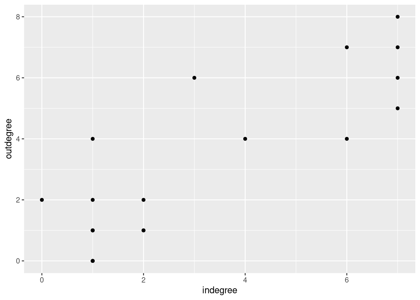
Changing Aesthetics for Everything
We can change things about the points by adding other arguments to geom_point() (there are a lot of options, scroll to Aesthetics here to see them).
ggplot(df_out, aes(x = indegree, y = outdegree)) +
  geom_point(color = "steelblue4", size = 6)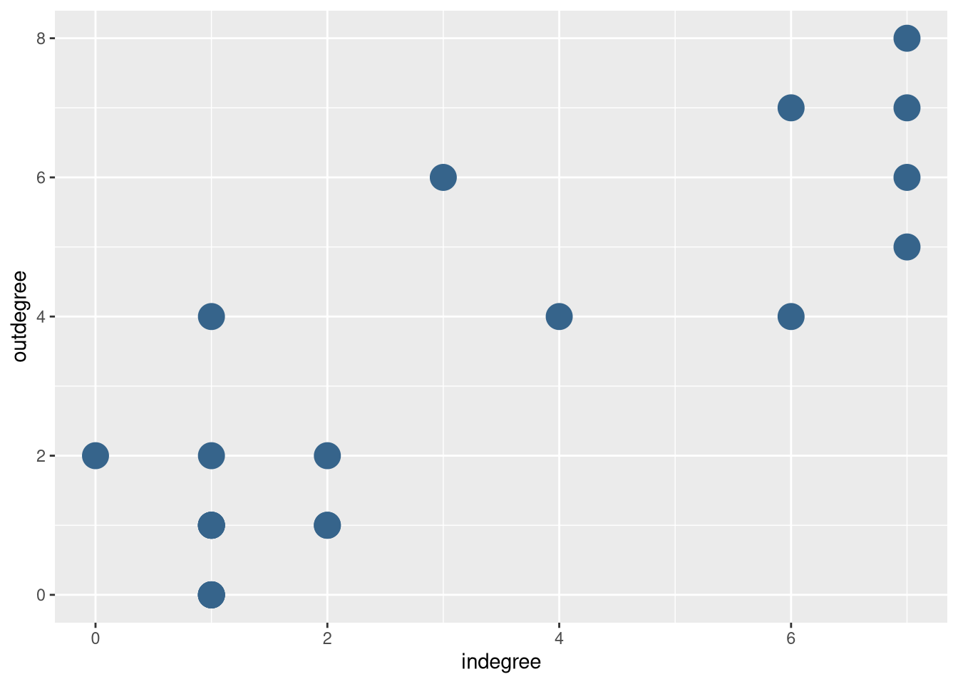
Changing Aesthetics for Some Things
We can also use the aes() function within the geom_point() call to have different aesthetics mapped to our data. The below will change the color of the dots depending on whether they are a cutpoint or not.
ggplot(df_out, aes(x = indegree, y = outdegree)) +
  geom_point(aes(color = cuts), size = 6)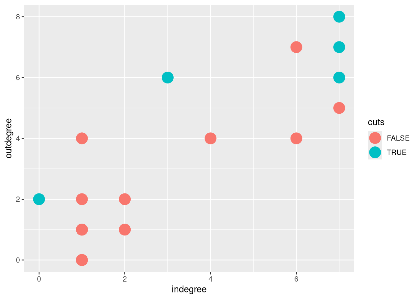
Changing Geoms
The power of ggplot are all the geoms. Lets change geom_point() to geom_jitter() which bumps around the dots, and add on another one: geom_smooth()` to show the trend.
ggplot(df_out, aes(x = indegree, y = outdegree)) +
  geom_jitter(aes(color = cuts), size = 6) +
  geom_smooth(method = "lm")
`geom_smooth()` using formula = 'y ~ x'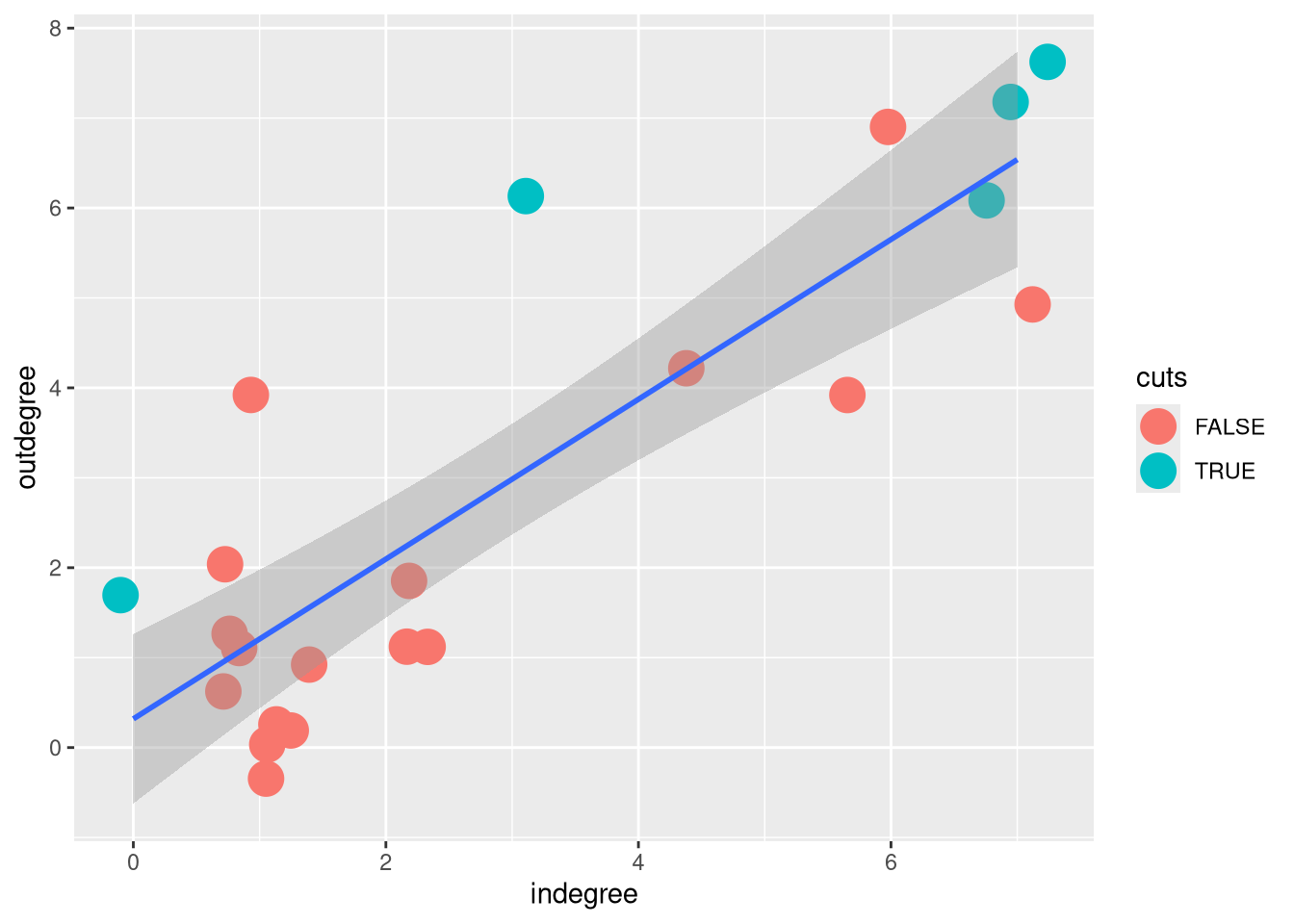
Where aes() is matters
Look what happens when you move the color=cuts part to the ggplot() call. Any aes() calls here impact all geoms.
ggplot(df_out, aes(x = indegree, y = outdegree, color = cuts)) +
  geom_jitter(size = 6) +
  geom_smooth(method = "lm")
`geom_smooth()` using formula = 'y ~ x'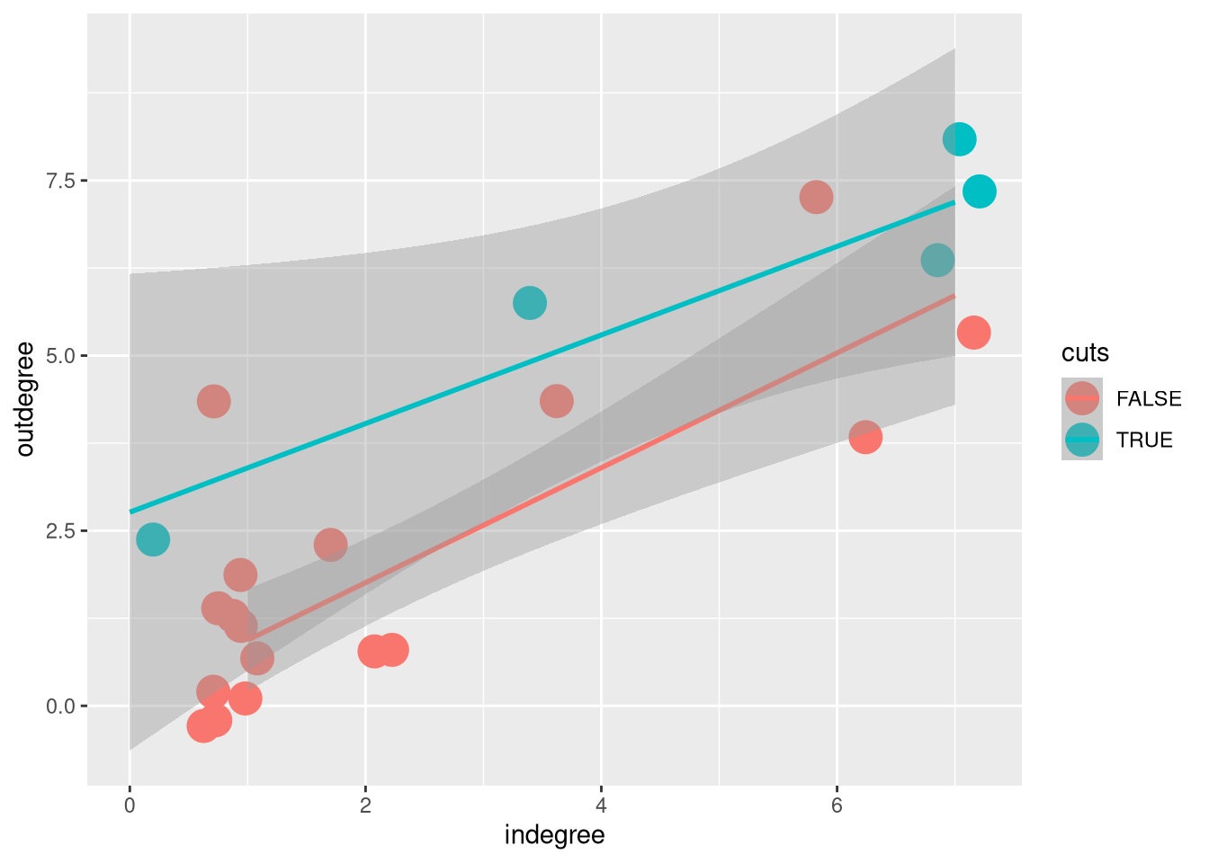
Adding Labels
We can add or modify labels to our plot using the labs() function
ggplot(df_out, aes(x = indegree, y = outdegree)) +
  geom_jitter(aes(color = cuts), size = 6) +
  geom_smooth(method = "lm") +
  labs(y = "Out Degree", x = "In Degree", title = "Out vs In Degree")
`geom_smooth()` using formula = 'y ~ x'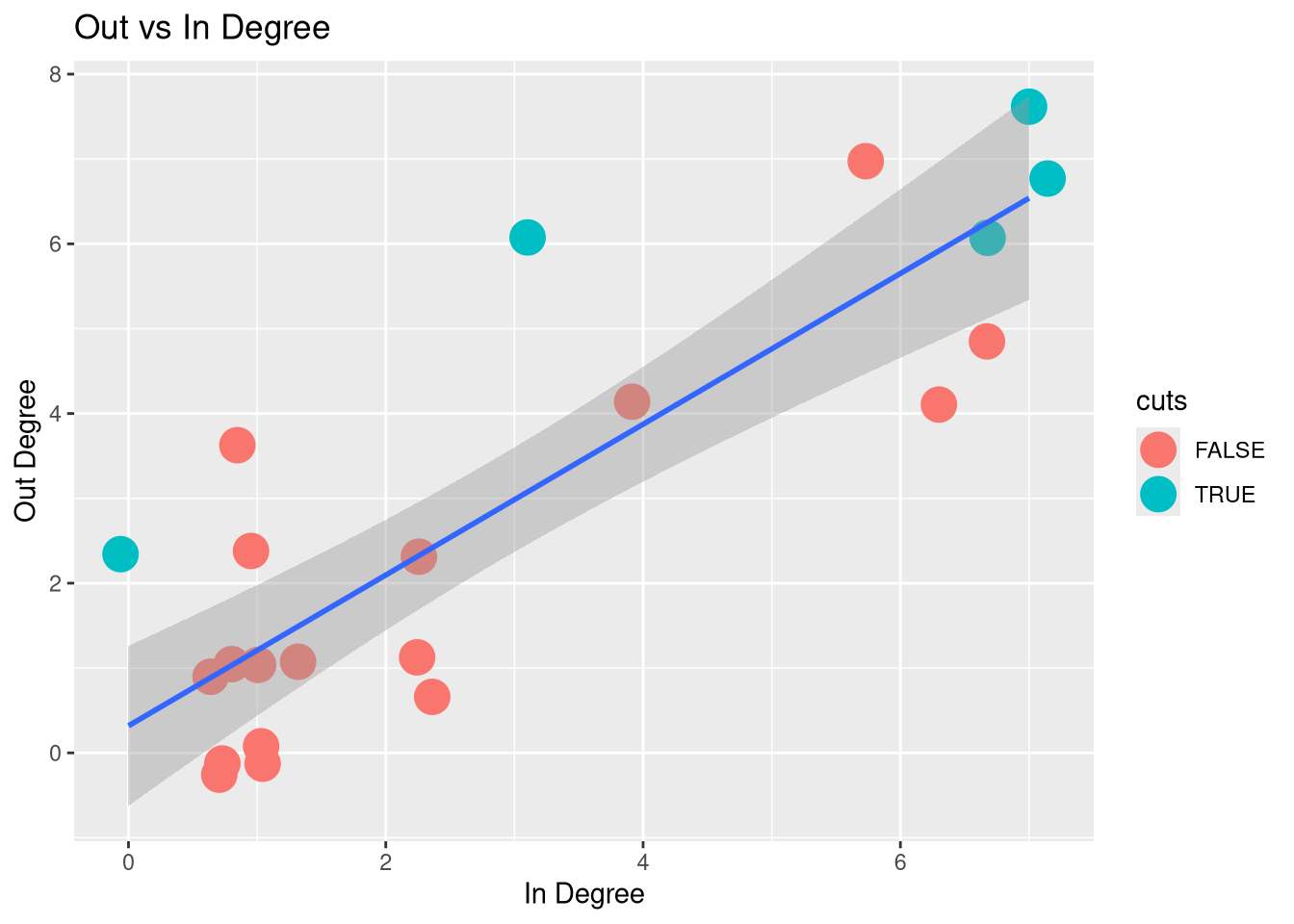
Editing the Scale
There are also scale_*_*() functions that can be used to change the style and labels of the scales.
ggplot(df_out, aes(x = indegree, y = outdegree)) +
  geom_jitter(aes(color = cuts), size = 6) +
  geom_smooth(method = "lm") +
  labs(y = "Out Degree", x = "In Degree", title = "Out vs In Degree") +
  scale_color_brewer("Cut Point?", type = "qual", palette = 2)
`geom_smooth()` using formula = 'y ~ x'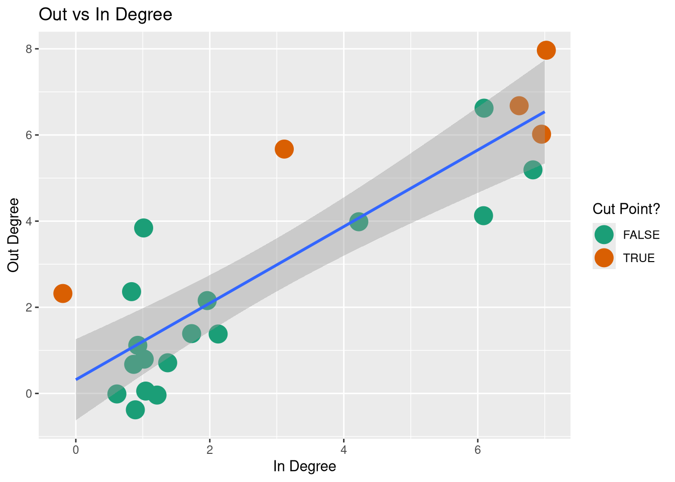
Themes
Finally you can use theme_*() to change the overall style of the plot
ggplot(df_out, aes(x = indegree, y = outdegree)) +
  geom_jitter(aes(color = cuts), size = 6) +
  geom_smooth(method = "lm") +
  labs(y = "Out Degree", x = "In Degree", title = "Out vs In Degree") +
  scale_color_brewer("Cut Point?", type = "qual", palette = 2) +
  theme_minimal()
`geom_smooth()` using formula = 'y ~ x'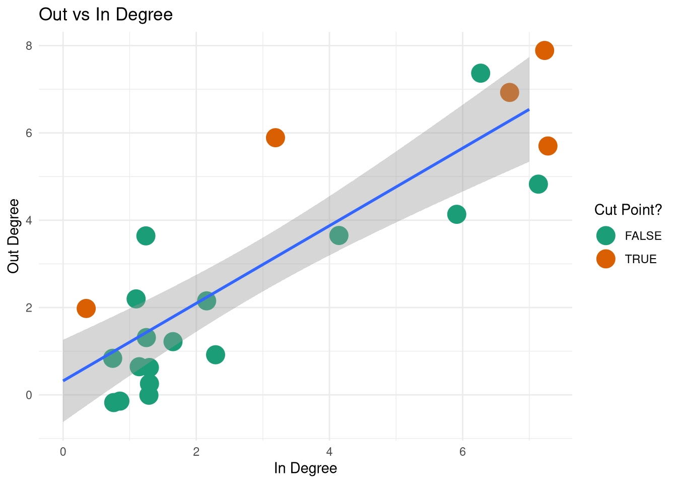
Footnotes
There are some who might write undirected matrices with only the upper or lower triangle filled, but this is not common.↩︎
The
#fmt: skipcomment is there because I use Air to format my code for consistency. This comment tells Air to not format the next line.↩︎