Visualizing Networks
Now we are going to move onto visualizing networks.
Visualizations can be useful with network data, but they are also hard to do:
We have complicated data.
We often want to show multiple “types” of information.
We are going to use the ggraph package.
Benefits:
It uses a ggplot2 style interface.
It allows a lot of fine-tuning of plots.
Has a fair amount of useful online documentation on layouts , nodes , and edges
Cons:
It is a bit overly complicated at times.
We are going to use a small canned dataset you can download from the internet: strike.paj
It is a communication network between workers at a sawmill. It also is a unique data format: “pajek” which thankfully igraph has a function for
Attaching package: 'igraph'
The following objects are masked from 'package:stats':

    decompose, spectrum
The following object is masked from 'package:base':

    union
<- read_graph (:: here ("resources/network_data/strike.paj" ),format = "pajek"
Warning in read_graph_pajek_impl(instream = file): Skipping unknown section '*Partition' on line 68.
Source: src/vendor/cigraph/src/io/pajek-lexer.l:130
Basics of Plot
Just like ggplot2 all visualizations will start with a call to ggraph()
Loading required package: ggplot2
theme_set (theme_graph ())ggraph (net)
Using "stress" as default layout
Warning: Existing variables `x` and `y` overwritten by layout variables
Adding Nodes and Edges
To add nodes and edges to this plot we will use geom_node_point() and geom_edge_link()
geom_node_point: Adds our nodes as circlesgeom_edge_link: Adds edges as straight lines (no arrows)
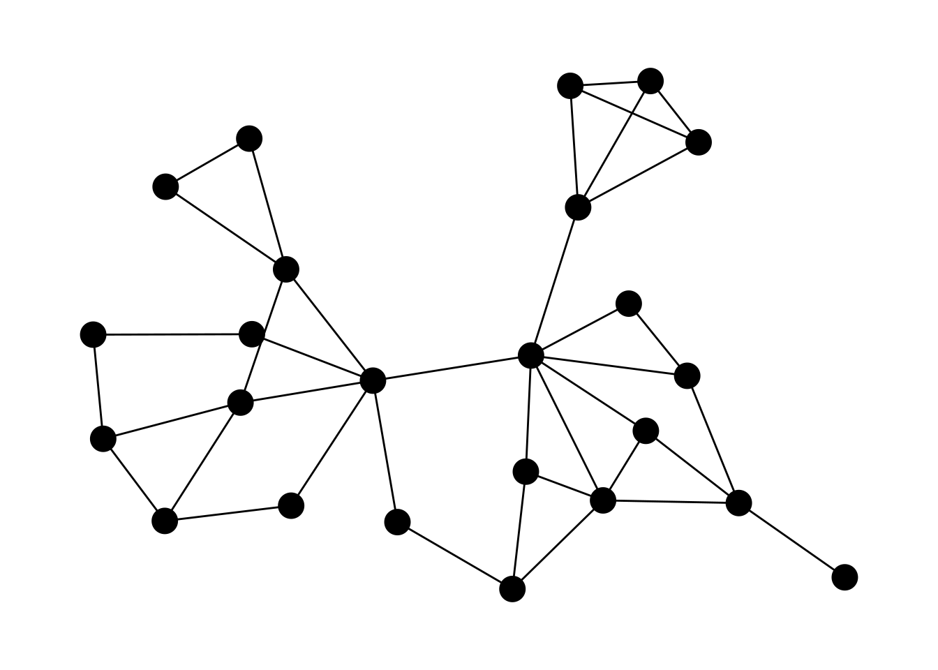
ggraph (net) + geom_node_point (size = 6 ) + geom_edge_link ()
Using "stress" as default layout
Warning: Existing variables `x` and `y` overwritten by layout variables
Layouts
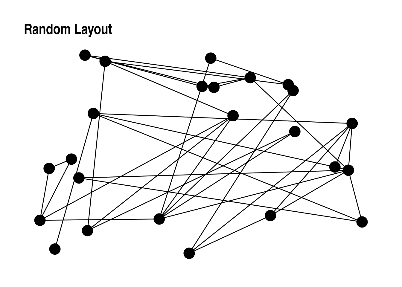
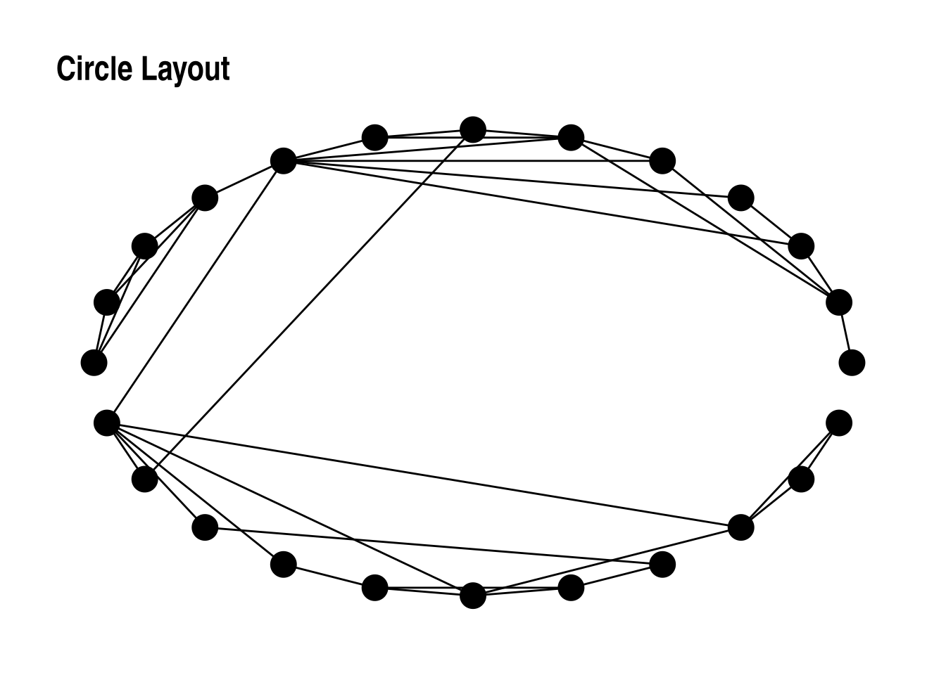
Laying out a plot can impact how useful it is by a lot:
Warning: Existing variables `x` and `y` overwritten by layout variables
Warning: Existing variables `x` and `y` overwritten by layout variables
Layouts Two Broad Approaches:
Dimension Reduction: Use multivariate techniques to scale into two dimensions
MDS, Pivot Scaling, Eigenvector
Force-Directed: Simulates a physical process
Fruchterman and Reingold, Kamada and Kawai, Davidson-Harel, DrL, Large Graph Layout (LGL), Graphopt, and GEM
Force-Directed
In most of these layouts they do something like:
Each node repulses all other nodes.
Edges pull two nodes together.
The balance of this is that groups of nodes with lots of connections are close and groups without them are far.
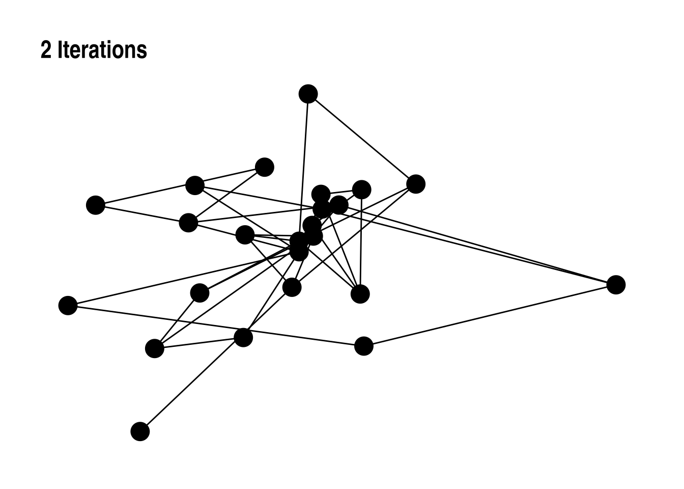
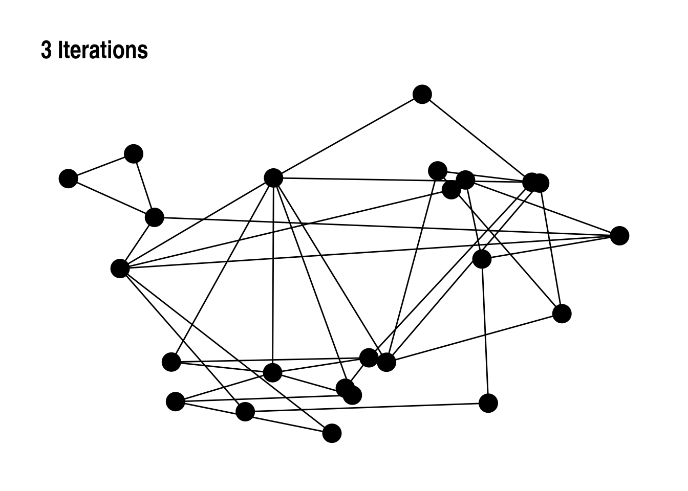
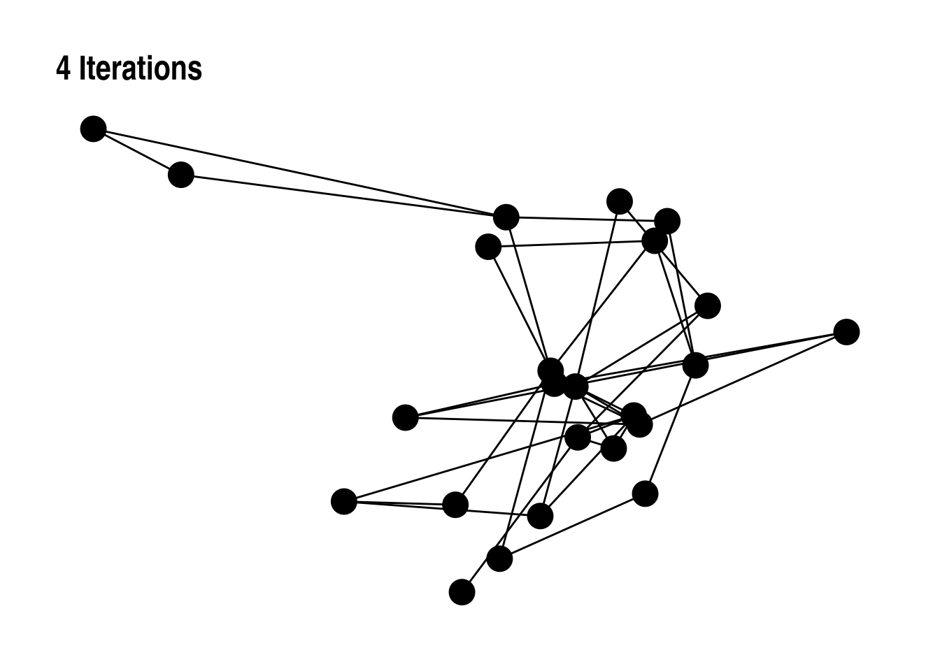
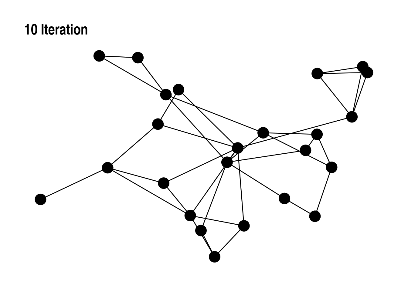
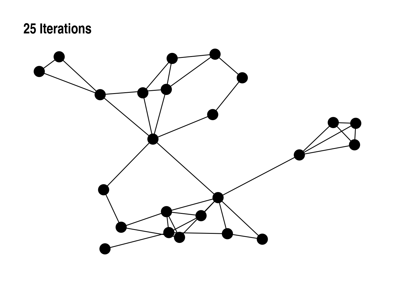
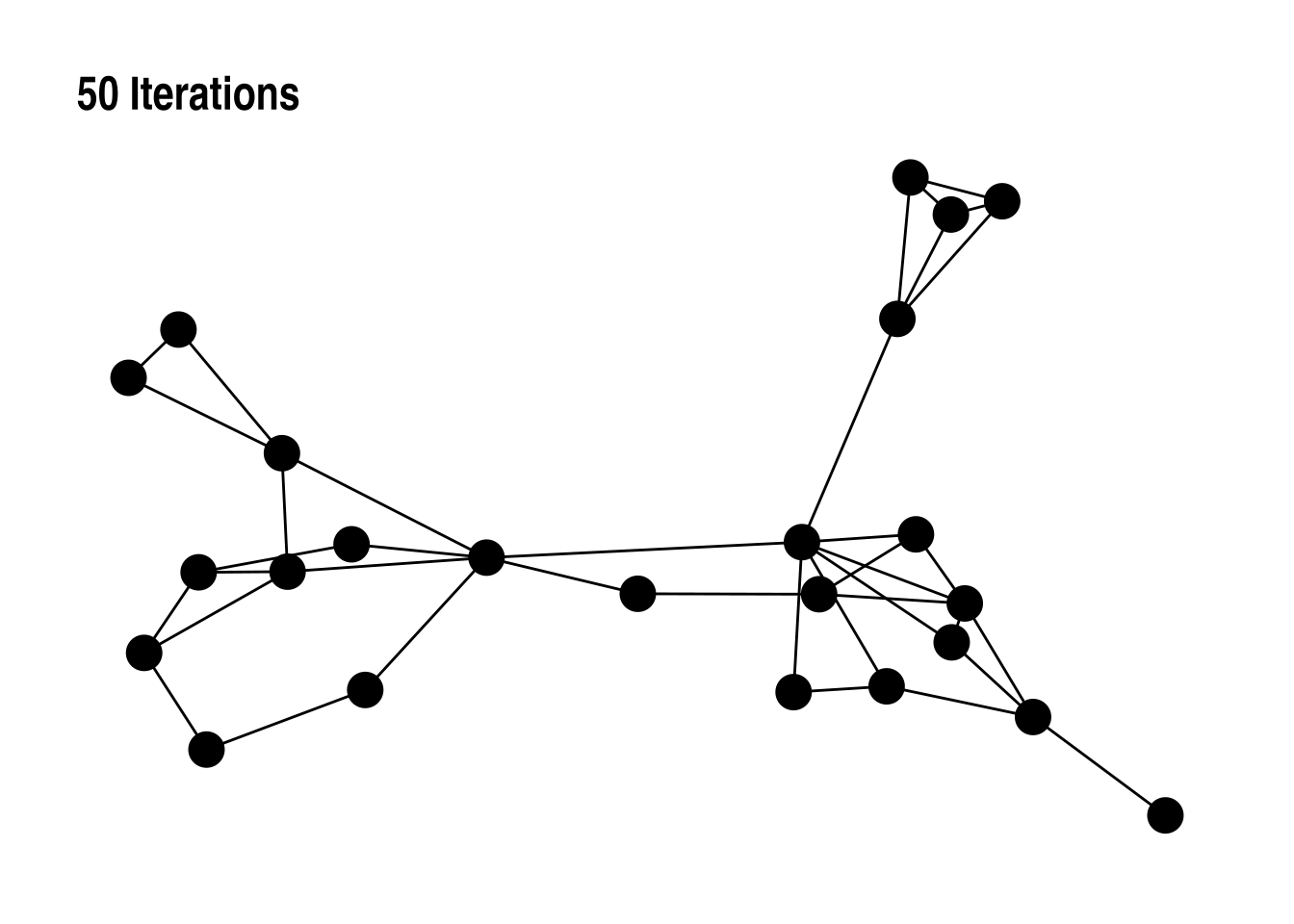
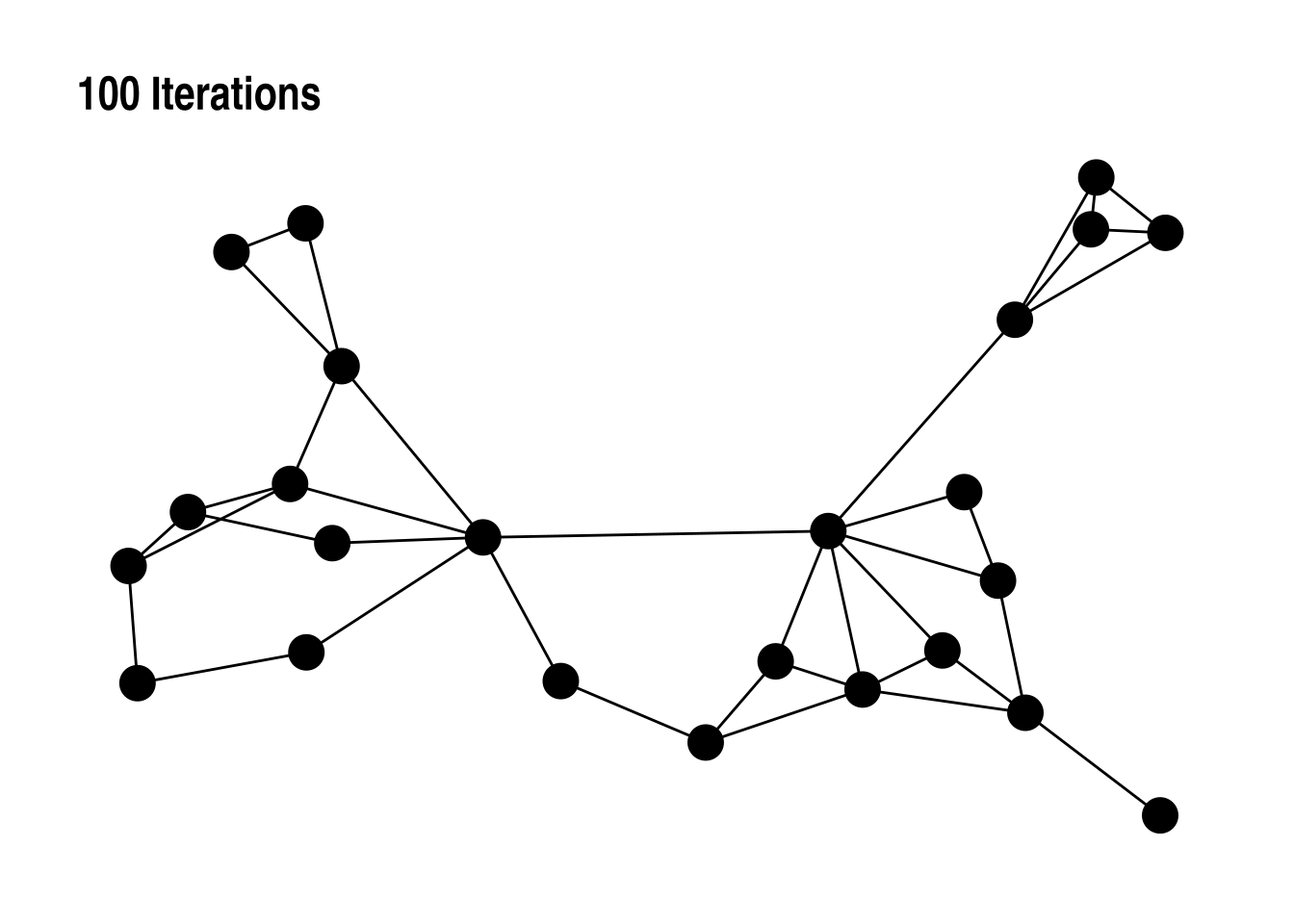
Fruchterman and Reingold Example
FR views vertexes as “atomic particles or celestial bodies, exerting attractive and repulsive forces from one another”.
How does this algorithm work?
Calculate the amount of repulsion between all nodes.
Calculate the amount of attraction between all adjacent nodes.
Move nodes based on the weight of attraction and repulsion, but limit the amount of movement by a temperature .
Reduce the temperature , go back to step 1.
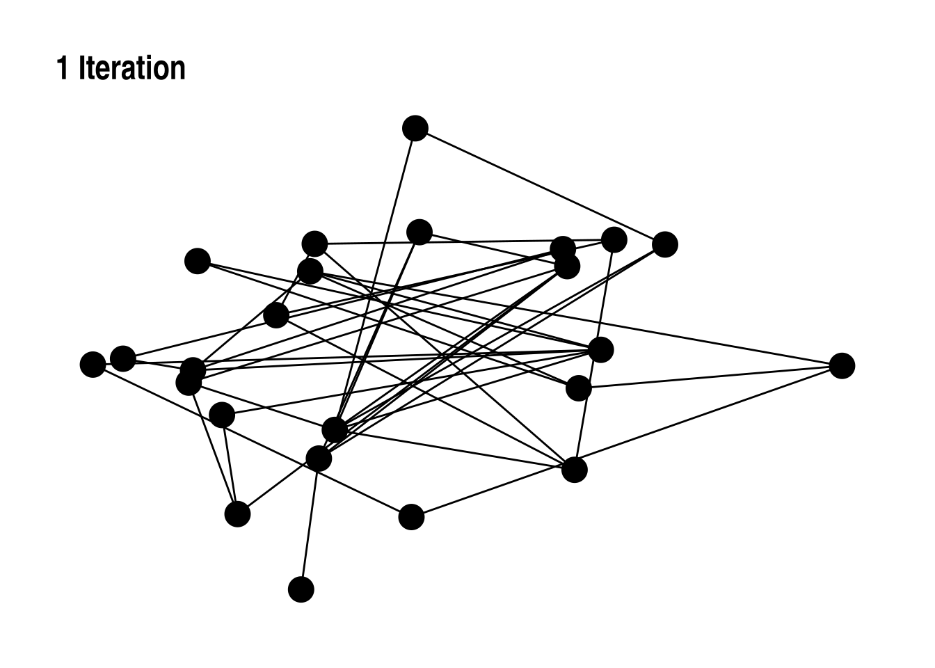
Fruchterman and Reingold Example
set.seed (1 )<- create_layout (net, layout = "igraph" , algorithm = "fr" , niter = 1 )ggplot (lo) + geom_node_point (size = 6 ) + geom_edge_link () + labs (title = "1 Iteration" )set.seed (1 )<- create_layout (net, layout = "igraph" , algorithm = "fr" , niter = 2 )ggplot (lo) + geom_node_point (size = 6 ) + geom_edge_link () + labs (title = "2 Iterations" )set.seed (1 )<- create_layout (net, layout = "igraph" , algorithm = "fr" , niter = 3 )ggplot (lo) + geom_node_point (size = 6 ) + geom_edge_link () + labs (title = "3 Iterations" )set.seed (1 )<- create_layout (net, layout = "igraph" , algorithm = "fr" , niter = 4 )ggplot (lo) + geom_node_point (size = 6 ) + geom_edge_link () + labs (title = "4 Iterations" )set.seed (1 )<- create_layout (net, layout = "igraph" , algorithm = "fr" , niter = 10 )ggplot (lo) + geom_node_point (size = 6 ) + geom_edge_link () + labs (title = "10 Iteration" )set.seed (1 )<- create_layout (net, layout = "igraph" , algorithm = "fr" , niter = 25 )ggplot (lo) + geom_node_point (size = 6 ) + geom_edge_link () + labs (title = "25 Iterations" )set.seed (1 )<- create_layout (net, layout = "igraph" , algorithm = "fr" , niter = 50 )ggplot (lo) + geom_node_point (size = 6 ) + geom_edge_link () + labs (title = "50 Iterations" )set.seed (1 )<- create_layout (net, layout = "igraph" , algorithm = "fr" , niter = 100 )ggplot (lo) + geom_node_point (size = 6 ) + geom_edge_link () + labs (title = "100 Iterations" )
Setting Layouts
To set the layout you set layout= to what you want, you can also pass additional arguments as necessary.
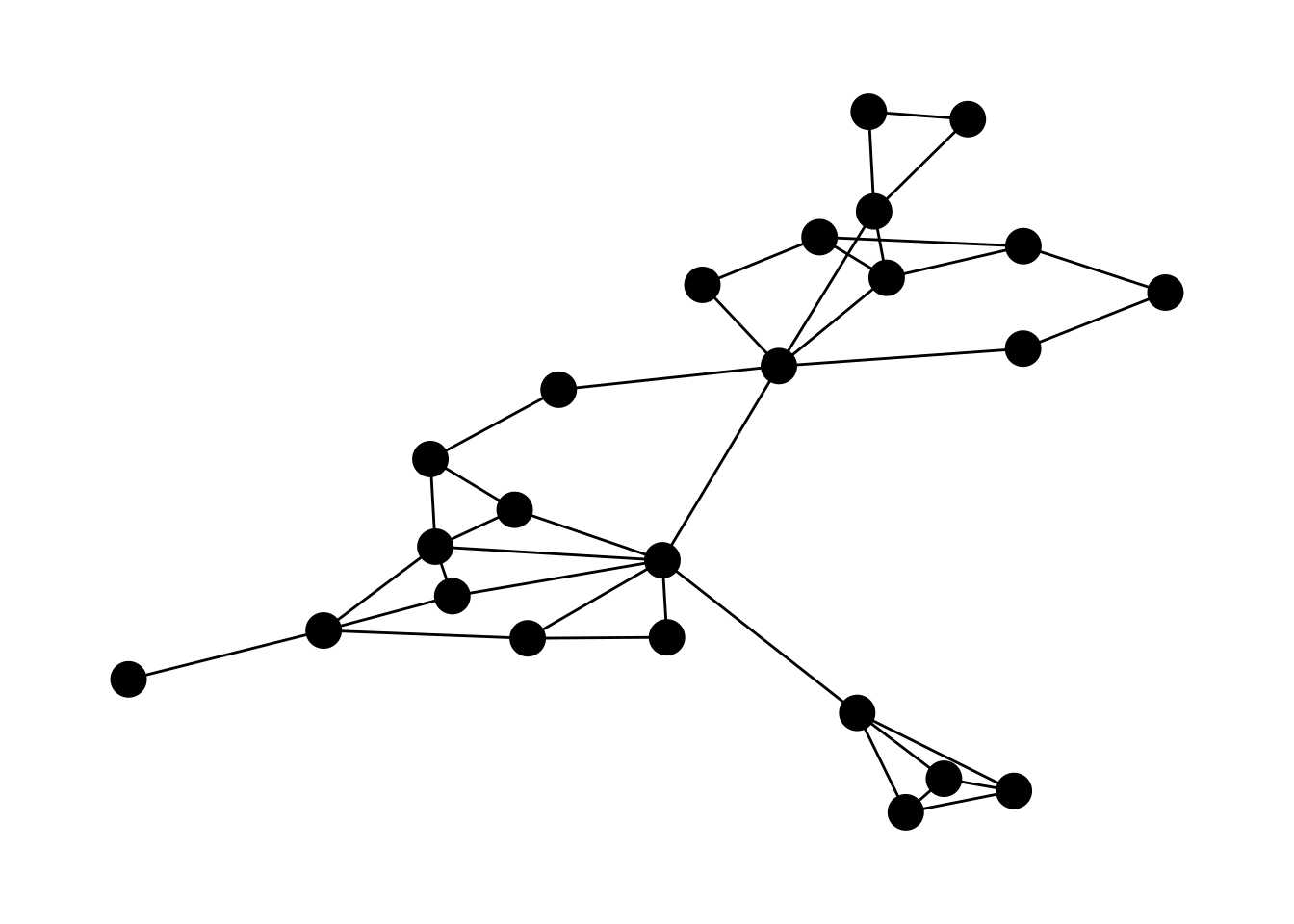
If you want to create the exact same layout every time run set.seed() directly prior to making the plot. This sets the “random seed” that is used.
set.seed (1 )ggraph (graph = net, layout = "fr" , niter = 250 ) + geom_edge_link () + geom_node_point (size = 6 )
Warning: Existing variables `x` and `y` overwritten by layout variables
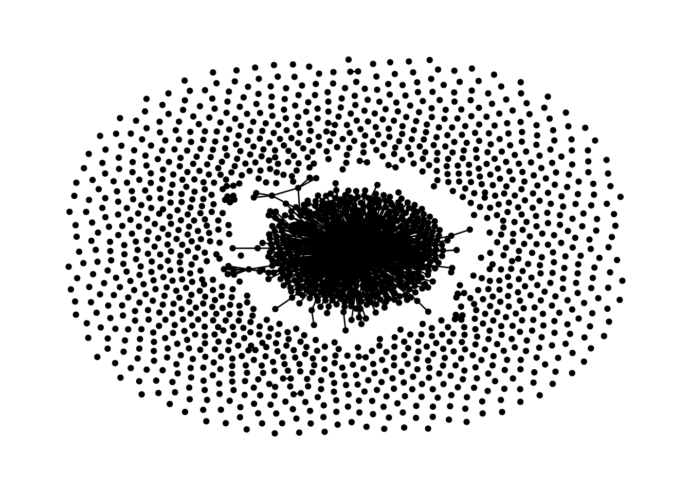
Large Network - DNC
Network of DNC emails from here.
<- read_graph (:: here ("resources/network_data/dnc.gml" ),format = 'gml'
Warning in read_graph_gml_impl(instream = file): One or more unknown entities will be returned verbatim (
).
Source: io/gml.c:150
ggraph (graph = dnc_net, "graphopt" ) + geom_edge_link () + geom_node_point ()
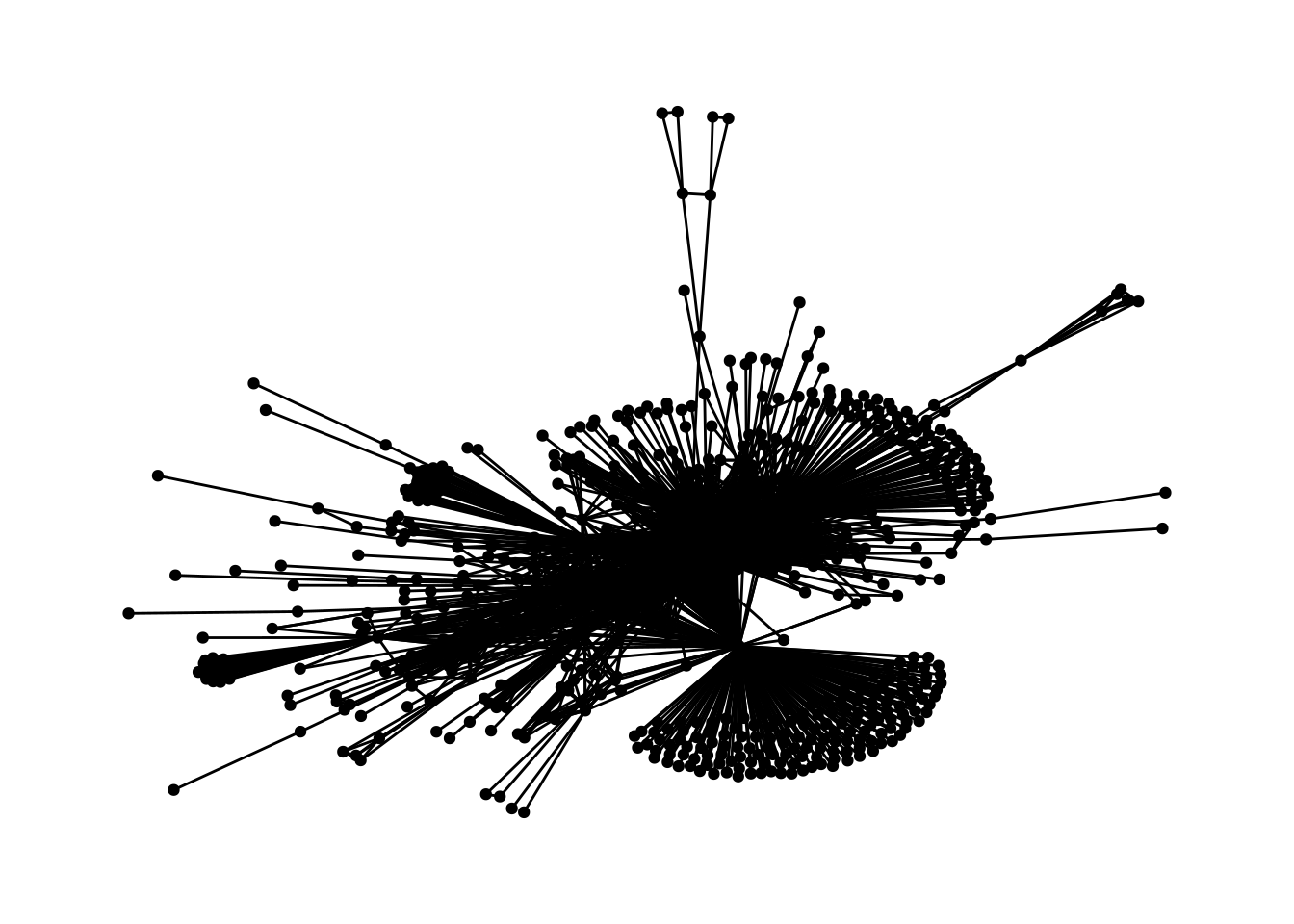
Large Network - Only Main Component
We can use the function largest_component() to grab just that part. Also the |> is a pipe which passes on the output.
|> largest_component () |> ggraph ("fr" ) + geom_edge_link () + geom_node_point ()
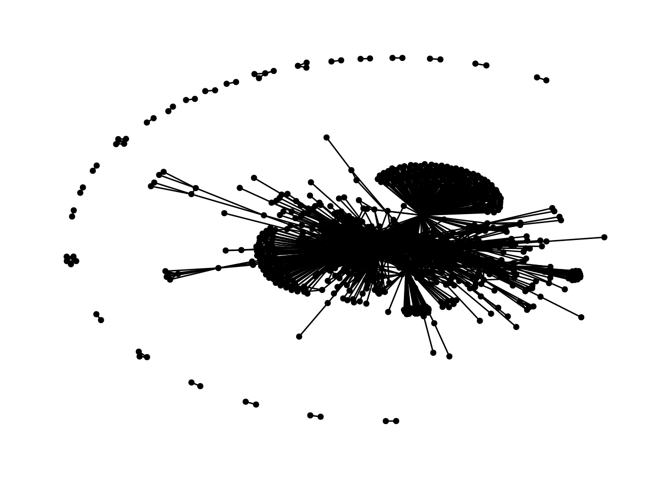
Large Network - No Isolates
Deleting all the isolates using which() and delete_vertices().
<- which (igraph:: degree (dnc_net) == 0 )|> delete_vertices (v = isolates) |> ggraph ("fr" ) + geom_edge_link () + geom_node_point ()
Labeling Nodes
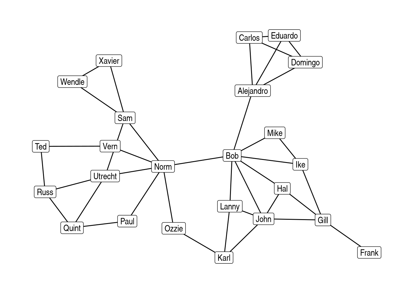
We can use geom_node_text() or geom_node_label() to label our nodes.
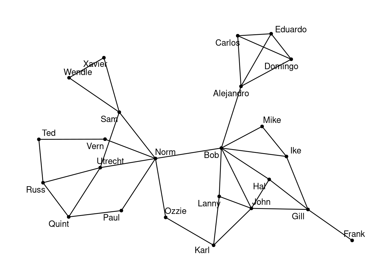
ggraph (graph = net, "stress" ) + geom_edge_link () + geom_node_label (aes (label = name))
Warning: Existing variables `x` and `y` overwritten by layout variables
They also have a repel=T argument that will move the labels away from the center of the node.
ggraph (graph = net, "stress" ) + geom_edge_link () + geom_node_point () + geom_node_text (aes (label = name), repel = T)
Warning: Existing variables `x` and `y` overwritten by layout variables
Vertex Attributes
Vertex attributes are included for a variety of reasons. This includes:
Demonstrating who is important in a network.
Showing groups in a network.
Presenting other relevant details.
Scaling by Degree
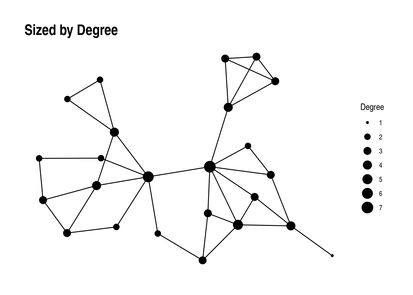
Often we will scale a node size by a measure of importance, like degree:
V (net)$ degree <- igraph:: degree (net)ggraph (graph = net, "stress" ) + geom_edge_link () + geom_node_point (aes (size = degree)) + ggtitle ("Sized by Degree" ) + scale_size ("Degree" )
Warning: Existing variables `x` and `y` overwritten by layout variables
New Network
This data is of Spanish high school students and includes negative and positive relations. We are going to delete the negative edges.
<- read.csv (here:: here ("resources/network_data/spanish_hs_edges.csv" ))<- read.csv (here:: here ("resources/network_data/spanish_hs_nodes.csv" ))<- graph_from_data_frame (edges, vertices = nodes, directed = T)<- which (E (net)$ weight < 0 )<- delete_edges (net, neg_edges)
IGRAPH 6c6c06c DNW- 105 1058 --
+ attr: name (v/n), Colegio (v/n), Curso (v/n), Grupo (v/c), Sexo
| (v/c), prosocial (v/n), crttotal (v/n), X_pos (v/c), id (e/n), weight
| (e/n)
+ edges from 6c6c06c (vertex names):
 [1] 3043->3047 3043->3087 3043->3093 3043->3065 3043->3097 3043->3044
 [7] 3043->3045 3043->3088 3043->3056 3043->3090 3043->3073 3043->3066
[13] 3043->3060 3043->3092 3043->3096 3043->3077 3043->3084 3043->3105
[19] 3043->3067 3043->3064 3043->3081 3043->3068 3043->3061 3043->3058
[25] 3043->3055 3043->3072 3043->3095 3043->3051 3043->3054 3043->3086
[31] 3043->3085 3043->3089 3043->3047 3043->3048 3043->3049 3043->3050
+ ... omitted several edges
Coloring Vertices
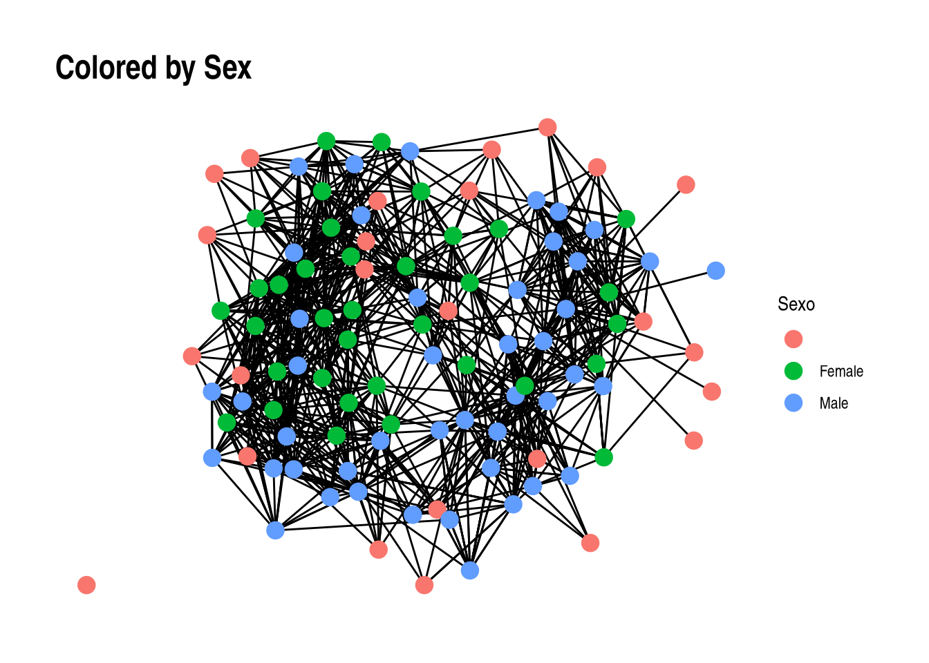
We can color the nodes by setting aes(color=) to a vertex attribute.
ggraph (graph = net, "stress" ) + geom_edge_link () + geom_node_point (aes (color = Sexo), size = 4 ) + ggtitle ("Colored by Sex" )
Edges
There are a few things we might want to do with our edges:
Add arrows for a directed network.
Show edge attributes.
General
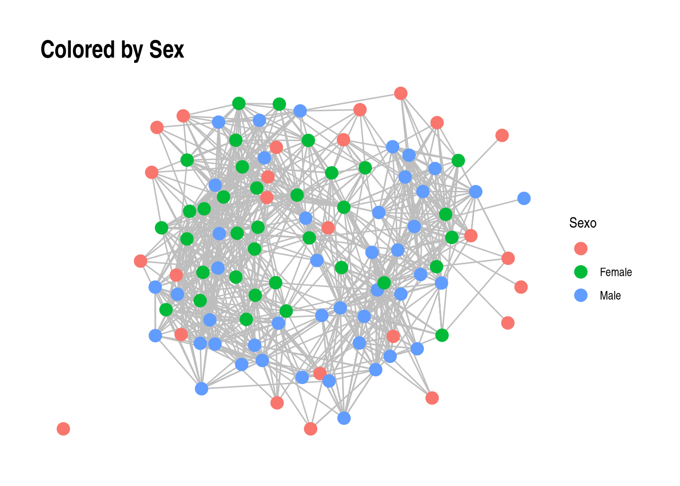
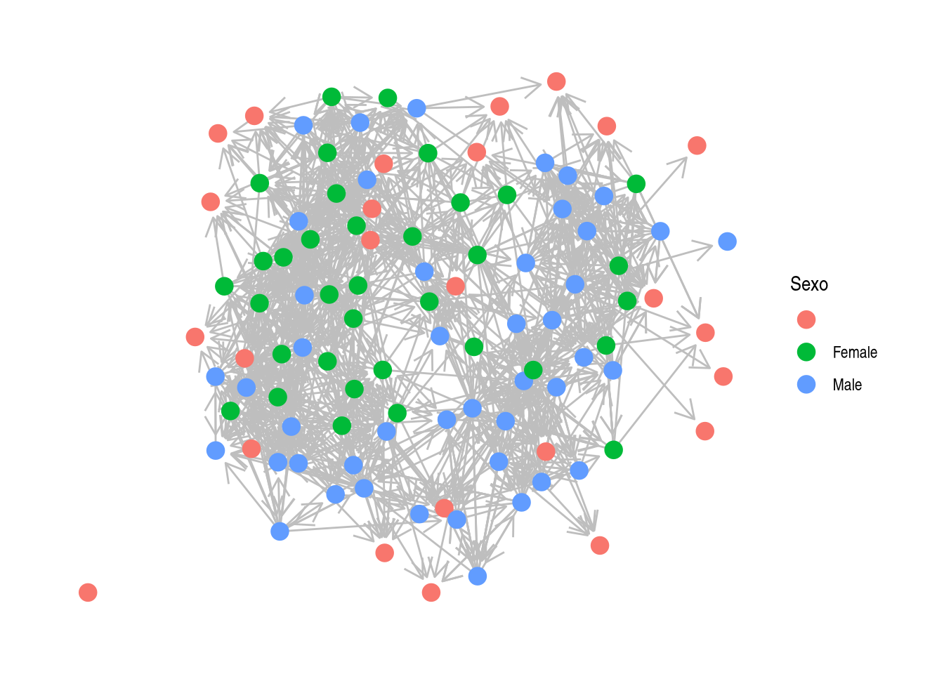
I think it is easier to see a network by making the edges gray.
ggraph (graph = net, "stress" ) + geom_edge_link (color = "gray" ) + geom_node_point (aes (color = Sexo), size = 4 ) + ggtitle ("Colored by Sex" )
Adding Arrows
Arrows are annoying to add here, but there is some good help online . We manually create an arrow (arrow) and manually end them before the node (end_cap)
ggraph (graph = net, "stress" ) + geom_edge_link (color = "gray" ,arrow = arrow (length = unit (4 , 'mm' )),end_cap = circle (3 , 'mm' )+ geom_node_point (aes (color = Sexo), size = 4 )
Adding Attributes
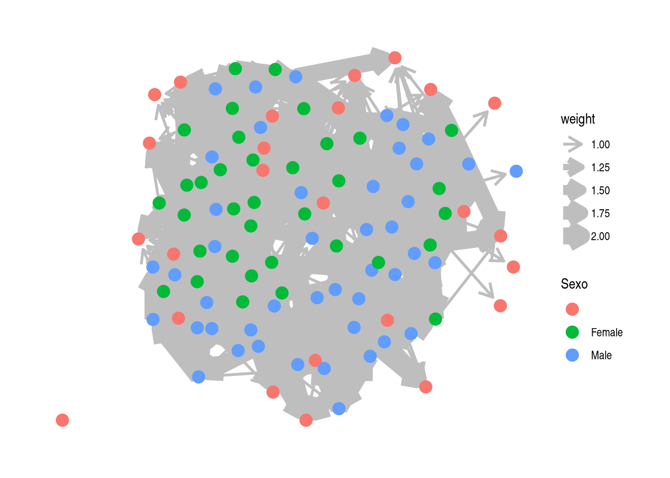
Finally we can assign edge attributes to aesthetics
ggraph (graph = net, "stress" ) + geom_edge_link (color = "gray" ,aes (width = weight),arrow = arrow (length = unit (4 , 'mm' )),end_cap = circle (3 , 'mm' )+ geom_node_point (aes (color = Sexo), size = 4 )
Warning: The `trans` argument of `continuous_scale()` is deprecated as of ggplot2 3.5.0.
ℹ Please use the `transform` argument instead.
Multiple
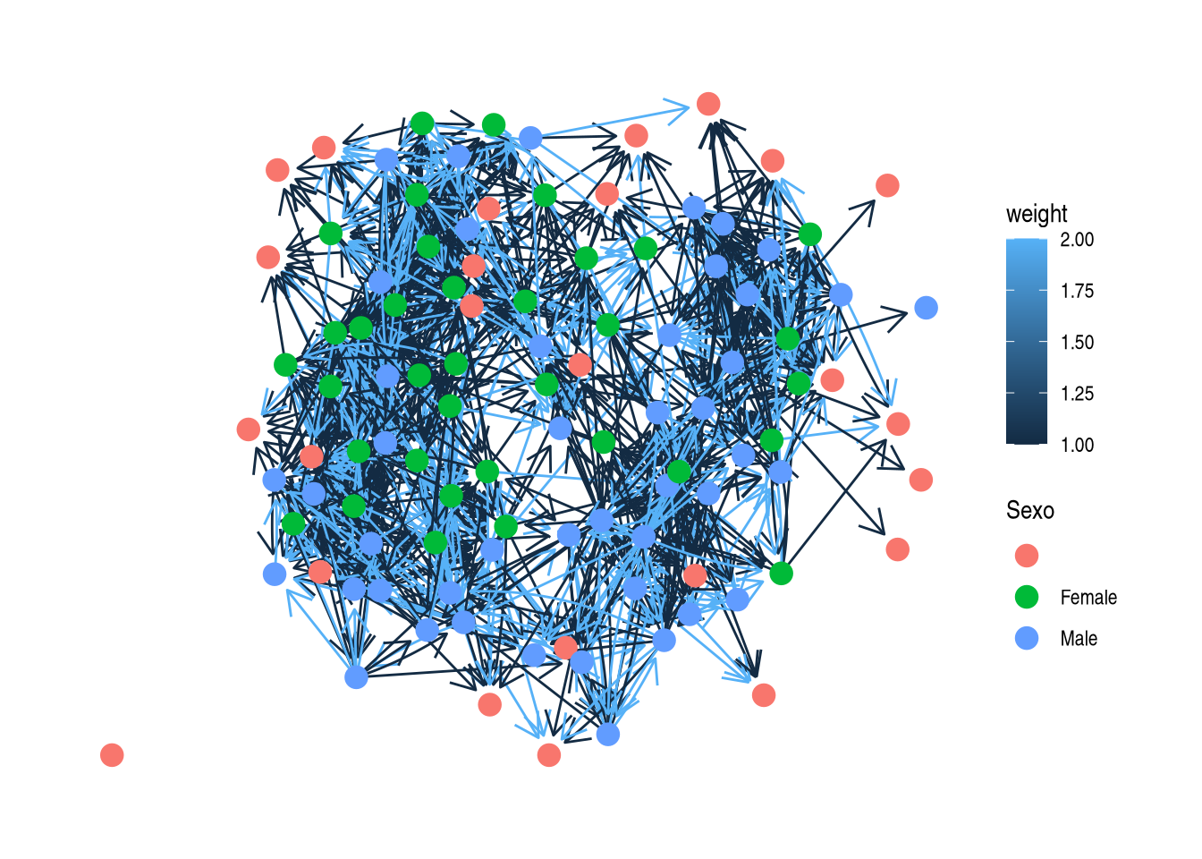
The default for ggraph is to show only a single edge when there are two mutual edges. We can change that by using geom_edge_fan()
ggraph (graph = net, "stress" ) + geom_edge_fan (aes (color = weight),arrow = arrow (length = unit (4 , 'mm' )),end_cap = circle (3 , 'mm' )+ geom_node_point (aes (color = Sexo), size = 4 )