| A | B | |
|---|---|---|
| 1 | Strongly Agree | Agree |
| 2 | Agree | Agree |
| 3 | Neither | Neither |
| 4 | Disagree | Disagree |
| 5 | Strongly Disagree | Disagree |
| 6 | Don't Know | Neither |
Recoding Data with xlookup
Google Sheets
POL 307
We often need to recode survey data meaning that we want to replace values with a different response. For example, we might have Strongly Agree, Agree, Neither, Disagree, Strongly Disagree and we want to group all the types of Agree into one category and the Disagree into another category.
There are a variety of ways to do this, and here we are going to learn how to use xlookup() in Google Sheets/Excel.
xlookup in general
xlooup is used when you want to fill in information into a cell based on the value in another cell. It follows the pattern:
XLOOKUP(search_key, lookup_range, result_range, missing_value, match_mode, search_mode)
The search_key will be what you are searching for, the lookup_range will be where you are looking for the search_key, and the result_range will be where it grabs things to return. The lookup_range and the result_range have to have an equivalent number of rows1 so if the search_key is found in row 3 of the lookup_range then it returns the 3rd row of the result_range.
To make this slightly clearer, Table 1 shows what could be your result_range and lookup_range for the prompt we started with. The lookup_range is in column A, while the result_range is in column B. When checking for “Agree”, xlookup finds it in A2 which is the second row of the lookup_range and so returns the second row of the result_range (B2)
All this means is that in order to use xlookup you have to first create a “codebook” table where your lookup and return values are matched in someway. I often like to do this on a different tab of the Google Sheet as to keep the data tab clean.
Using xlookup
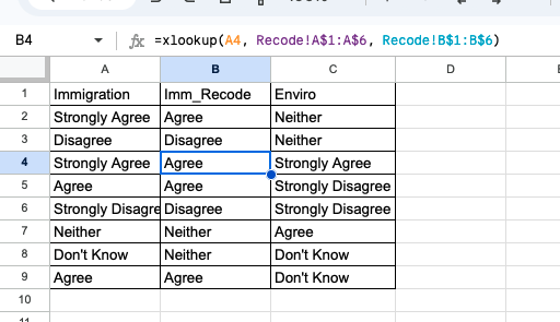
In Table 2 I show what this would look like in practice. Here I assume that Table 2 (b) is in a second tab of your Google Sheet labeled Recode. The formula used is: =xlookup(A2, RecodeA$1:A$6, RecodeB$1:B$6)2. If you wanted to do the same recoding process for the Enviro column you just need to change A2 to C2 and go from there.
| A | B | C | |
|---|---|---|---|
| 1 | Immigration | Imm_Recode | Enviro |
| 2 | Strongly Agree | =xlookup(A2, Recode!A$1:A$6, Recode!B$1:B$6) | Neither |
| 3 | Disagree | =xlookup(A3, Recode!A$1:A$6, Recode!B$1:B$6) | Neither |
| 4 | Strongly Agree | =xlookup(A4, Recode!A$1:A$6, Recode!B$1:B$6) | Strongly Agree |
| 5 | Agree | =xlookup(A5, Recode!A$1:A$6, Recode!B$1:B$6) | Strongly Disagree |
| 6 | Strongly Disagree | =xlookup(A6, Recode!A$1:A$6, Recode!B$1:B$6) | Strongly Disagree |
| 7 | Neither | =xlookup(A7, Recode!A$1:A$6, Recode!B$1:B$6) | Agree |
| 8 | Don't Know | =xlookup(A8, Recode!A$1:A$6, Recode!B$1:B$6) | Don't Know |
| 9 | Agree | =xlookup(A9, Recode!A$1:A$6, Recode!B$1:B$6) | Don't Know |
| A | B | |
|---|---|---|
| 1 | Strongly Agree | Agree |
| 2 | Agree | Agree |
| 3 | Neither | Neither |
| 4 | Disagree | Disagree |
| 5 | Strongly Disagree | Disagree |
| 6 | Don't Know | Neither |
Figure 2 shows what this would look like on Google Sheets. Again, assuming that you have a second tab.
Replacing numbers with categories
In a lot of cases we want to take continuous data and collapse it into categories. For example, you might want to create age buckets out of ages, replacing 41 with “31-49”. To do this we need to use the match_mode argument mentioned above.
match_mode controls the rules used for matching your data. The default (0) will only match if things are exactly the same. We can also set it to 1, and -1. I think the rules for these are a bit hard to parse but here is the language from Google:
1is for an exact match or the next value that is greater than thesearch_key.
-1is for an exact match or the next value that is lesser than thesearch_key.
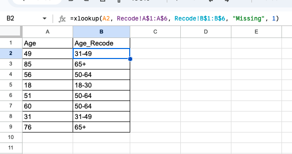
This means that if you select 1, it will search for the search_key in your lookup table. If it does not find that exact number it will select the cell that is close to your search_key but greater than your search_key. In Table 3 the first age is 49, which is exactly in A2 of the recoding so it matches with the second row. The second age is 85 which is not in the recode table so the next step is to match with the value that is the next largest number above 85. This is 120 in cell A4, and so the fourth row is matched. You should pay attention to this, and always double check with a few known values.
One final note, in order to set the match_mode we also have to set the missing_value argument. The missing_value argument is simply what it returns when it cannot find the missing value. Below I’ve used "Missing" but this could be anything.
In total our formula is then: =xlookup(A2, Recode!A$1:A$6, Recode!B$1:B$6, "Missing", 1)
| A | B | |
|---|---|---|
| 1 | Age | Age_Recode |
| 2 | 49 | =xlookup(A2, Recode!A$1:A$6, Recode!B$1:B$6, "Missing", 1) |
| 3 | 85 | =xlookup(A3, Recode!A$1:A$6, Recode!B$1:B$6, "Missing", 1) |
| 4 | 56 | =xlookup(A4, Recode!A$1:A$6, Recode!B$1:B$6, "Missing", 1) |
| 5 | 18 | =xlookup(A5, Recode!A$1:A$6, Recode!B$1:B$6, "Missing", 1) |
| 6 | 51 | =xlookup(A6, Recode!A$1:A$6, Recode!B$1:B$6, "Missing", 1) |
| 7 | 60 | =xlookup(A7, Recode!A$1:A$6, Recode!B$1:B$6, "Missing", 1) |
| 8 | 31 | =xlookup(A8, Recode!A$1:A$6, Recode!B$1:B$6, "Missing", 1) |
| 9 | 76 | =xlookup(A9, Recode!A$1:A$6, Recode!B$1:B$6, "Missing", 1) |
| A | B | |
|---|---|---|
| 1 | 30 | 18-30 |
| 2 | 49 | 31-49 |
| 3 | 64 | 50-64 |
| 4 | 120 | 65+ |
Again, for those wanting to see this in Google Sheets, ?@fig-recode-numeric shows it.
Things I papered over
There are a few other things you can do with xlookup that aren’t useful for this class but are useful in general:
- You can actually have it return multiple cells. To do this you set your results range to have multiple rows.
- You can flip the orientation entirely and look up across rows instead of cells. The only really important rule here sit hat your lookup range can only be one column OR one row. Here we did one column, and so it assumed that this is the orientation you want to use.
Finally, xlookup is the newer version of vlookup and hlookup which are very similar but less flexible.