Rake Weights in Google Sheets

Google Sheets

POL 307

In this walkthrough we are going to learn rake weights in Google Sheets. This is not the easiest way to implement rake weights but you will have a much better idea of how they work by doing it this way. The hardest part of this is going to be preparing the Google Sheet. Once we have things prepared it will mainly be copying and pasting. Also thanks to Cory McCartan for providing an example of rake weights in Google Sheets.

We are going to do relatively simple weighting, targeting on sex and race.

Table 1: Targets

Attribute	Target
Female	0.5099
Male	0.4901
White	0.6102
Black	0.1199
Hispanic	0.1798
Other	0.0901

Gender - First Pass

Preparation

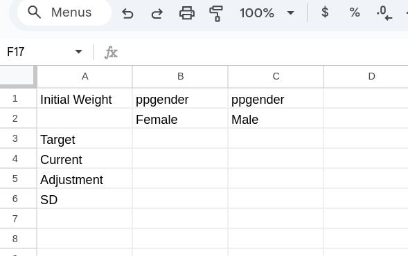
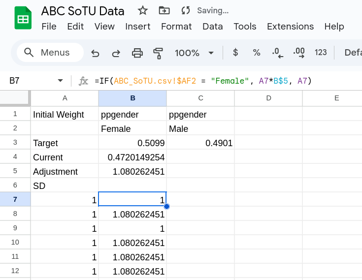
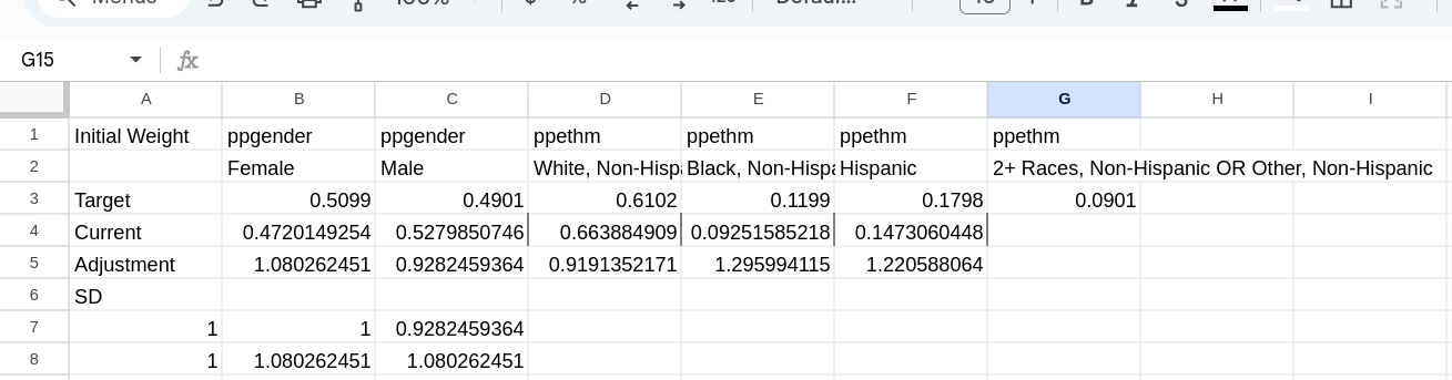
We will start by setting up a new tab. The furthest left column is going to be used as labels and our initial weights. We can put Initial Weight if we want at the top and then leave a space and put Target, Current, Adjustment, and SD below that on the left. In column two and three we are going to put the first two attributes we will weight to. This will be Female and Male in ppgender. This helps us to track what we are doing (see Figure 1).

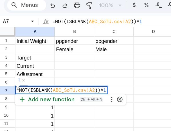
Next we are going to create our initial weights which will all just be 1. We are going to do this in a slightly complicated way but it will help to make sure that we aren’t accidentally creating data. What we will do is create an indicator for whether there is something in Response ID (we are picking this because it exists for every observation in our data) in each row. We can’t directly check whether a cell is filled but we can check whether a cell is not empty. This is the formula =NOT(ISBLANK(ABC_SoTU.csv!A2))¹. This will return TRUE for non-empty cells and FALSE for empty cells. We’d prefer just a 1 or a 0 so we will multiply that by *1 creating: =NOT(ISBLANK(ABC_SoTU.csv!A2))*1. Once you have that formula ready you can drag it down until you have a 0 showup. This should be around ~540 rows. For other data you might have to add additional rows. Delete any cells at the bottom that have a 0.

Next we need to add the target proportion and the current proportions. The target is easy as it is just the numbers in Table 1. In contract for the current we need an easy way to calculate the portion of our data that is Female (or Male). It will make our future life easier if we can incorporate our weights (which are all 1 currently). To do this we are going to use three functions nested within each other:

IF: Will allow us to check whether a cell contains our attribute of interest.
ARRAYFORMULA: We are going to apply the IF function to the entire variable at once. Normally Google Sheets would only return the first value, ARRAYFORMULA allows it to return multiple.
AVERAGE.WEIGHTED: Will calculate a weighted average of what we give it (which in this case will be the indicators for if a cell contains the attribute of interest or not).

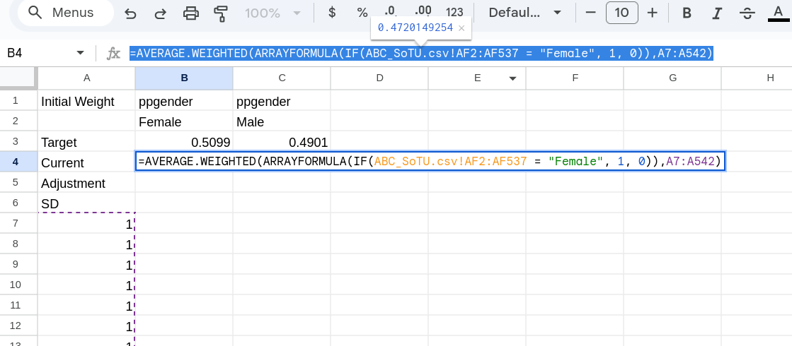
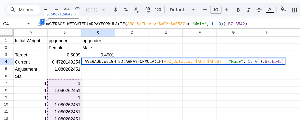
What we will write is something like: =AVERAGE.WEIGHTED(ARRAYFORMULA(IF(ABC_SoTU.csv!AF2:AF537 = "Female", 1, 0)),A7:A542). Moving from the inside out, the IF(ABC_SoTU.csv!AF2:AF537 = "Female", 1, 0) checks each individual cell from AF2:AF537 (yours will be different) is equal to the “Female” and returns 1 if it is or 0 if it isn’t. The ARRAYFORMULA(...) turns this into a single array. Finally the AVERAGE.WEIGHTED(... , A7:A542) calculates the average of those 1 and 0s weighted by the weights in A7:A542. If you’ve done everything right you should get a single number in that cell somewhere between 0 and 1 (what I have now is in Figure 3).

Note

The cells identified here are for the example data. In your homework you are going to have to make sure you’ve captured the whole column (you have more observations).

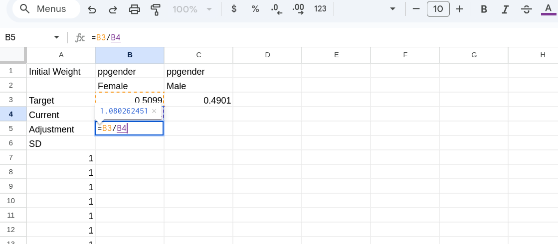
The final part of the preparation is calculating the adjustment. Remember this is just the $\frac{\text{Pop}}{\text{Sample}}$. In this case all we have to do then is put that into our excel in the adjustment row (see Figure 4)

Adjusting

Making the adjustment here will be easy. All we have to do is, for each row in our data, check whether ppgender is Female or not. If it is we adjust our base weight of 1, if it isn’t we just keep the base weight as it is. We want to set this up though with knowledge that we will eventually drag this to the right to use it for the Male category as well.

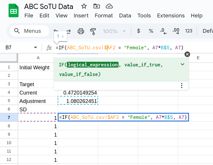
We will start then with the following formula =IF(ABC_SoTU.csv!$AF2 = "Female", A7*B$5, A7). In the IF() statement we check whether the first observation in the ppgender column is “Female” or not. If it is we then take the current weight (which is to the left) and multiply it by the adjustment (above). If it isn’t then we just pass over the weight. Note that we we lock the column we are pulling from in the original data, and the row the adjustment is in. See Figure 5.

Once we have that formula in place we can drag it down the row so we can make our adjustments for everything in the data (you don’t actually have to drag it, if you click on the cell and double click on the square in the bottom right it will fill in the rest of the column).

Switching to Male

Now that we’ve adjusted the Female rows we will switch to adjusting the Male rows. We will follow the same process: (1) calculating the current proportion, (2) calculating the adjustment, and (3) making the adjustment.

We could drag over the adjustment but before we do that we should lock the column we are checking (we could have done this prior). To do this we change the inside part to be: ARRAYFORMULA(IF(ABC_SoTU.csv!$AF2:$AF537 = "Female", 1, 0) (notice the $ before AF?). We can then copy it over to the Male column. We are going to update it in two ways then. First we change “Female” to “Male” and then we change the column we weight to from A.. to B… (we will copy this over later and want to have it just reference the column one before it so we don’t want to lock it).

The adjustment ratio is easy and we can just copy over the adjustment from the Female column (Figure 8).

Now we will adjust those who are “Male” in the ppgender column. To do this we can just copy over the adjustment we made in the Female column. All we have to do is change the ="Female" to ="Male". We will actually “adjust” the weights in the Female column, which might sound strange (shouldn’t we be adjusting the base weights?). It is fine though because our categories are mutually exclusive so we will only be adjusting weights that were not adjusted.

Race/Ethnicity - First Pass

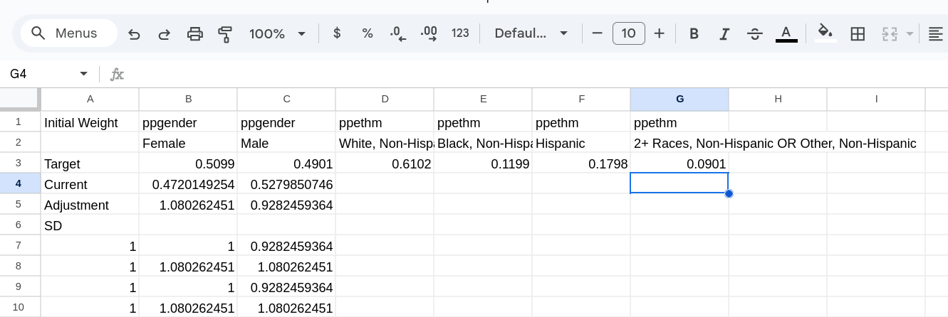
Now we are going to follow a similar process and adjust based on the attributes in ppethm. We can start again by putting in all our labels and targets. One thing that is a problem here is that the categories in the data don’t directly match our categories. There are actually 5 categories present in the data so we are going to have to use both “2+ Races, Non-Hispanic” and “Other, Non-Hispanic” when calculating our Other target/adjustment. You can add in all the information to the top 3 rows (Figure 10).

Creating Targets

We can start by creating our targets. This time we will create our targets and adjustments for all our categories first (either order is fine). The first three are easy to do and we just need to copy over the target calculation from the “Male” column and update a few things:

We need to change what column in the data we are checking (this will now be AE)
We need to update what we are checking (“White, Non-Hispanic”, “Black, Non-Hispanic”, “Hispanic”).
We need to make sure we are using our newly created weights in the Male column (we always want to use our newly adjusted weights once we move on to a new variable).

You should have something like Figure 11.

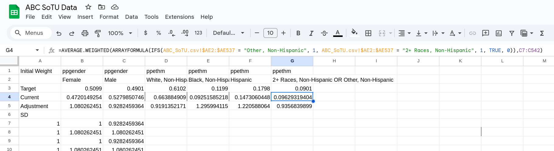
Checking whether a column is either “Other, Non-Hispanic” or “2+ Races, Non-Hispanic” is a bit more complicated. We will switch from using the IF() function to IFS() function. This function takes the form of IFS(X1, Y1, X2, Y2....). Each of the X* here are logical checks. It goes through each individually until one is true and then it will return the associated Y* value. We are going to write: IFS(ABC_SoTU.csv!$AE2:$AE537 = "Other, Non-Hispanic", 1, ABC_SoTU.csv!$AE2:$AE537 = "2+ Races, Non-Hispanic", 1, TRUE, 0) What this does is:

Checks if a value in the column is “Other, Non-Hispanic” and if so it returns 1
Checks if a value in the column is “2+ Races, Non-Hispanic” and if so it returns 1
Checks if TRUE is true (which is always true) and if so returns 0.

It does it in that order so the last check is a “if you’ve gotten this far return 1”.

We will replace the IF() with this and then have something like in Figure 12. We also can copy over the adjustment.

Making Adjustments

Now we need to make the adjustments of our weights. Again for the first three this is fairly easy. We can copy over formula we used to adjust the Male column and update it. All we have to change is what column in the data we are checking (AE remember) and what we are checking it for (“White, Non-Hispanic” in the first column)

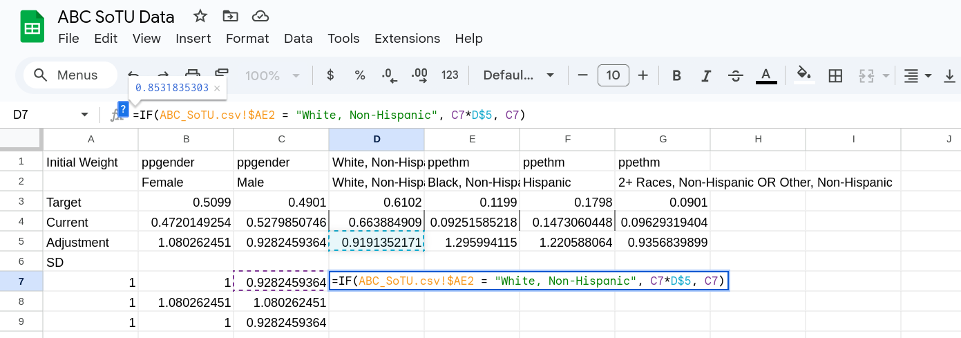
We can do that for the first three columns, filling in all the rows once we are done. We should now have Figure 14. You can notice that in each row we are again just multiplying by the adjustment if it fits the attribute we are checking against.

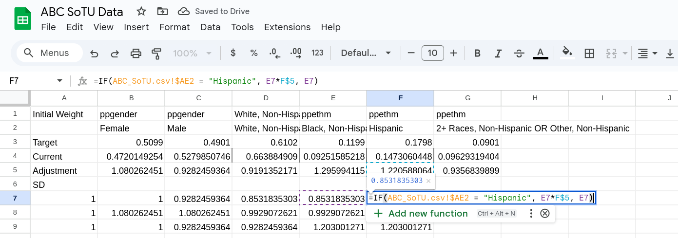
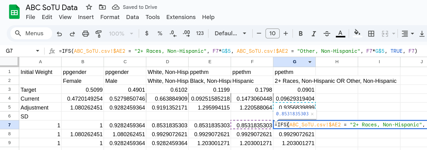
For our multi-attribute column we are again going to is IFS() where we check for each attribute separately and return the adjusted weight if it is true. If neither attribute is present we then return the original weight. This will look like: =IFS(ABC_SoTU.csv!$AE2 = "2+ Races, Non-Hispanic", F7*G$5, ABC_SoTU.csv!$AE2 = "Other, Non-Hispanic", F7*G$5, TRUE, F7) You can then fill the row in and it will look like Figure 15

Second Rake

At this point we have completed a single rake. The good thing is we don’t have to make any more manual changes to our sheet. All we have to do is copy all the columns associated with one pass of the rake, and then paste them in new columns to the right. Because of how we set things up (where it always uses the weight one to the left) it will continue the pattern.

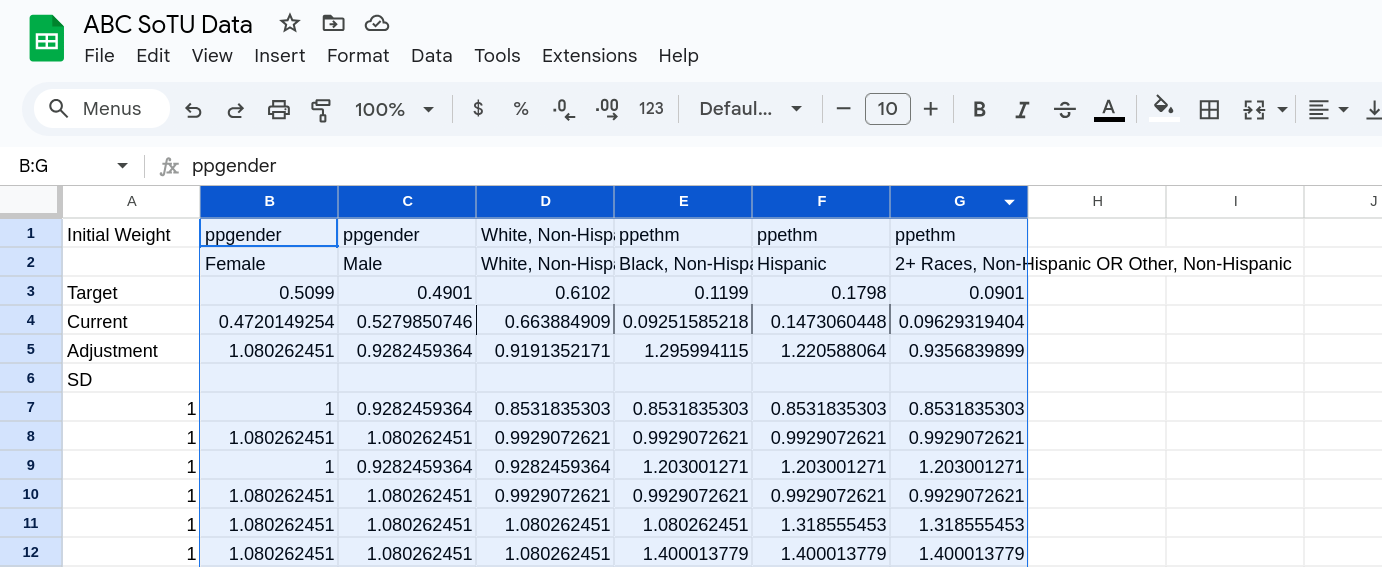
To do this just highlight the columns we’ve made (excluding the initial column) and copy it.

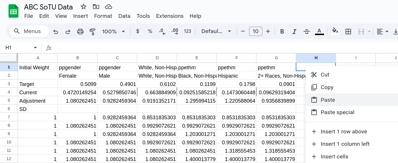
Then click in to the cell at the top of the first empty column and paste the results there (Figure 17).

Once you paste it you’ll see that the numbers update, and the adjustment factors should all be trending towards 1. Should paste it at least 4 times. This will create 5 rakes of your data.

Color Formatting Adjustment

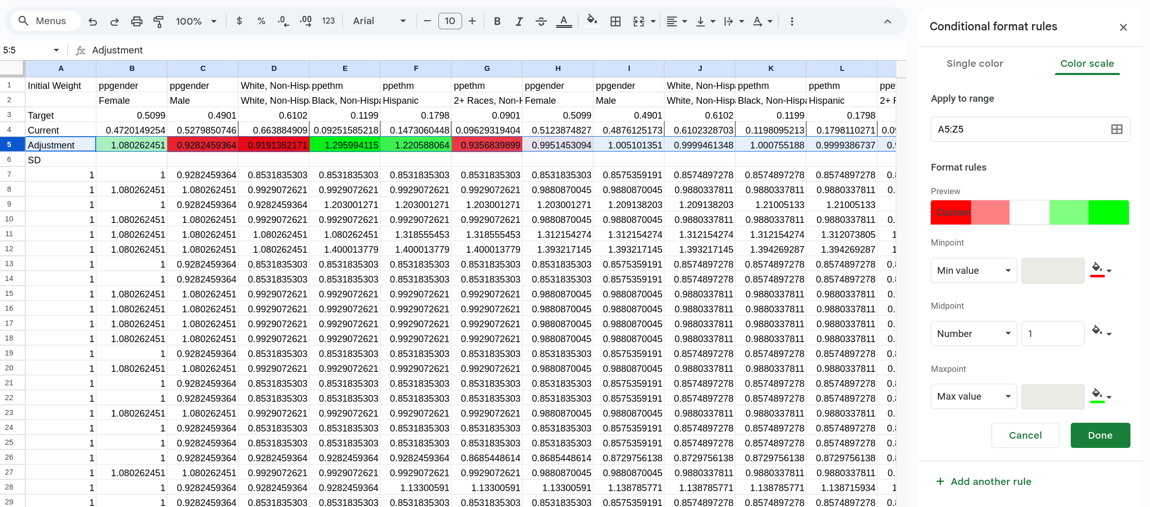
This isn’t necessary but if you want to see how the adjustment ratio changes you can turn on a conditional formatting of it. This formatting will change the color of the cells based on their value.

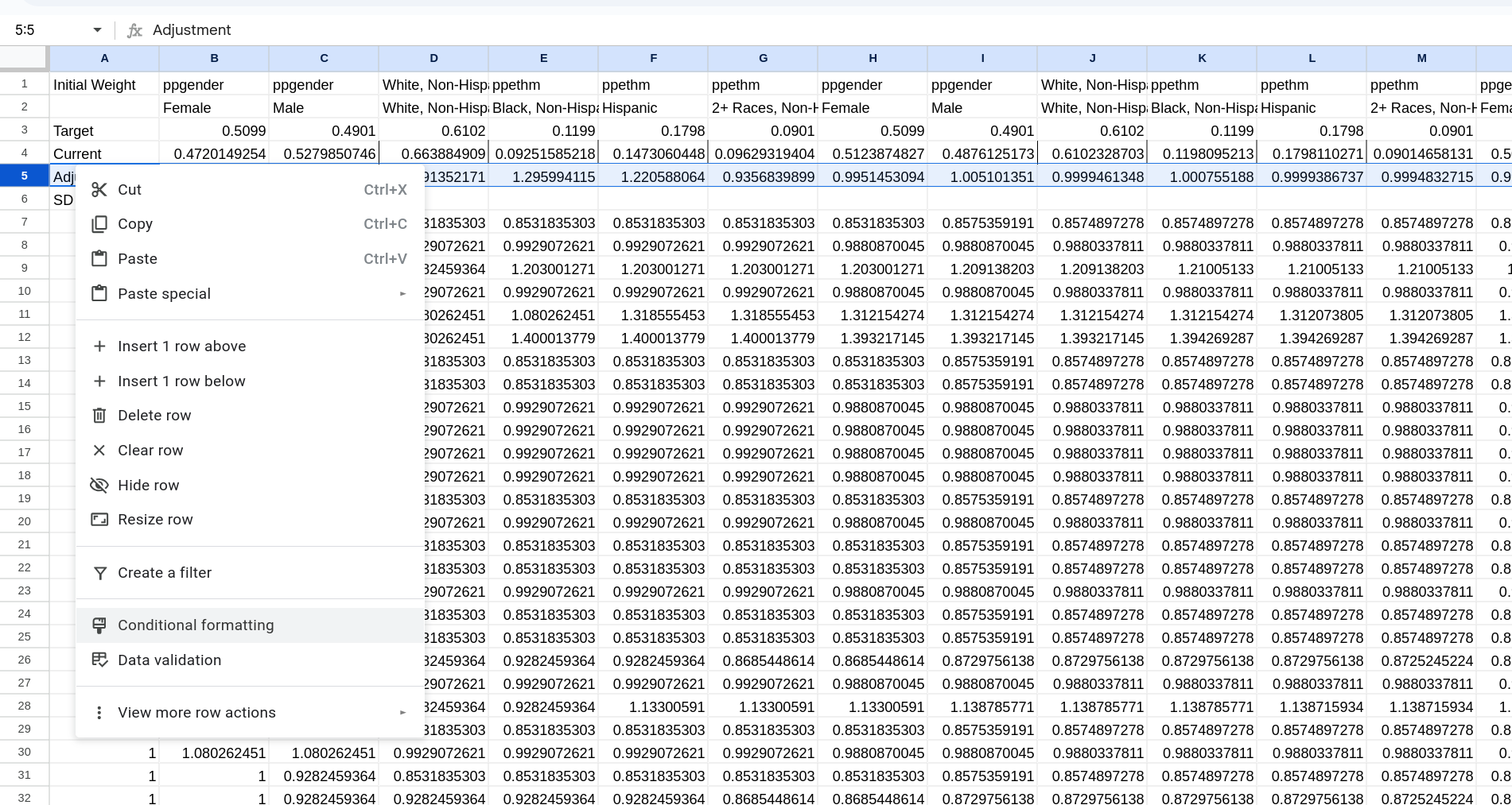
To do this highlight the whole row (by clicking the row label) and then right click and go to Conditional Formatting.

A menu will popup and you’ll switch it to Color Scale (at the top of the menu). You can then set the midpoint to a number (in the dropdown) and put in 1. If you want you can then change the colors of the different values. I like to set the midpoint to white (see Figure 18 for how I set this up).

Adding Our Weights to Our Data

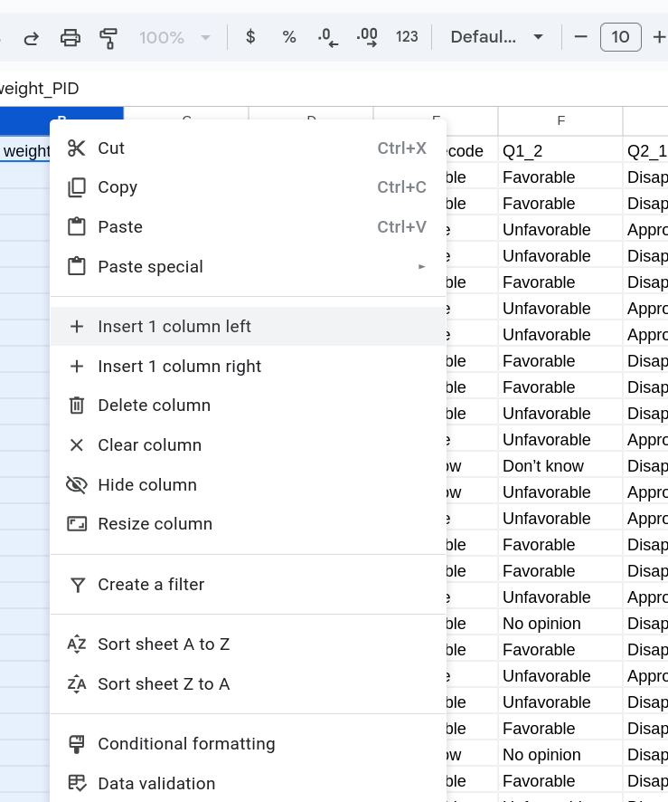
If we want to add our weights back to the data (to use in a pivot table) we can insert a new column into our data by right clicking on the column label (Figure 19) and selecting Insert 1 Column left.

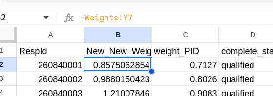
You can then label the column and use a formula to select the data from your weight table. For me this looks something like =Weights!Y7 (this formula is simple as we are just saying that this cell is the same as the other cell). Fill in this column and you’ll have your weights with your data.

Footnotes

You can click on the tab back to your data to then click Response ID in the very firsts row. The ABC_SoTU.csv is because that is the tab name that has the data for me.↩︎