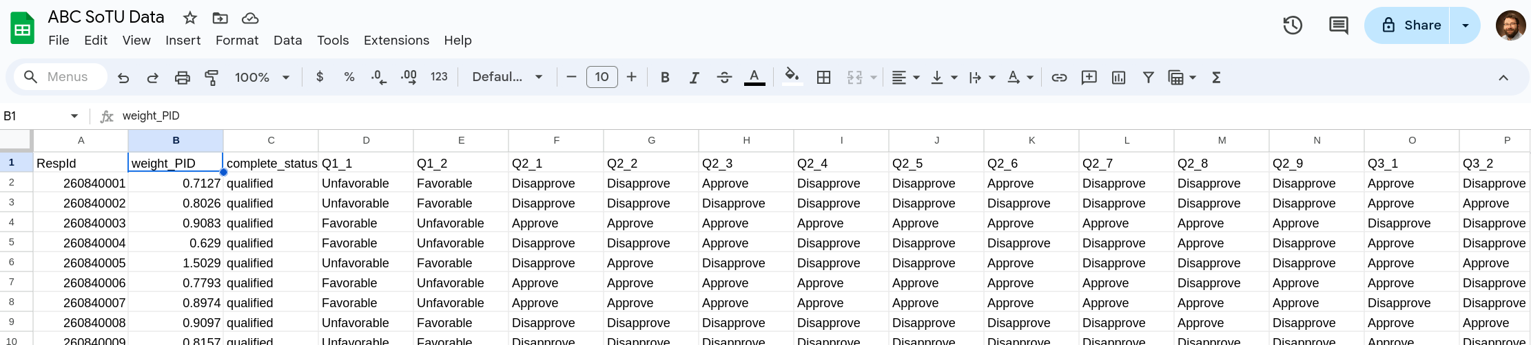
Univariate Stats in Google Sheets
Uploading Data
This tutorial is going to assume that you have a csv file already that you want to analyze. The easiest way to upload data is to start by creating a brand new Google Sheet document (see Figure 1).

Once you have created the new document you can go to File and then Open (Figure 2) to upload your csv file. A window will open and you select the Upload tab on the far right (Figure 3).


You should now have your CSV file opened in the Google Sheet. At this point you might consider changing the file name to something else by clicking the current name on the top left (it might have replaced this with the file name). You should be seeing something like Figure 4
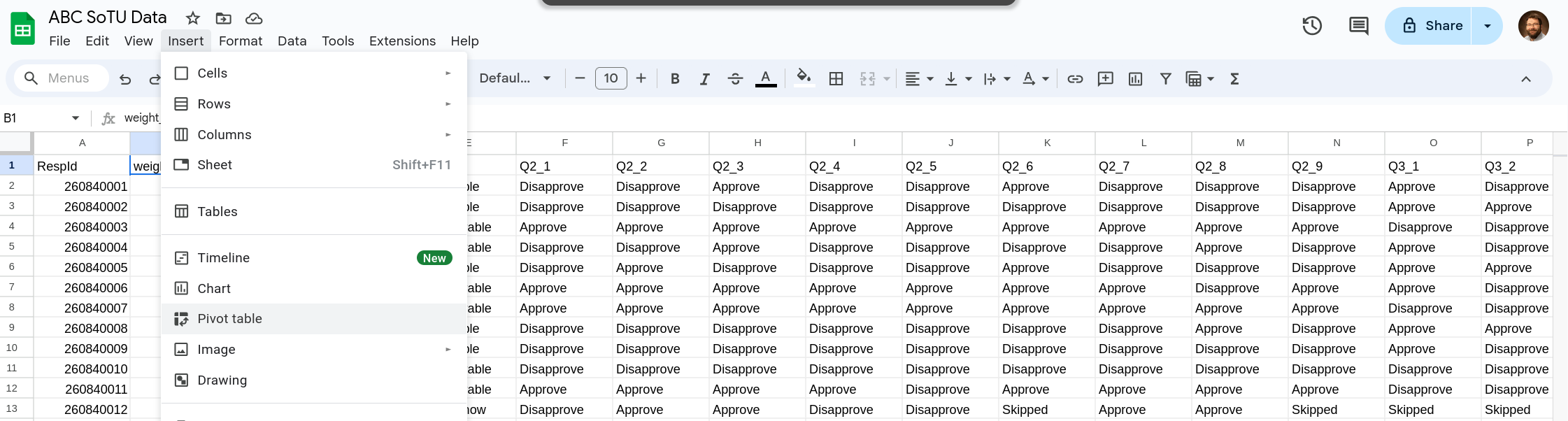
Creating A New Pivot Table
We will be using a pivot table to do our analysis. Pivot tables allow you to quickly aggregate your data in different ways and to create different aggregations for different groups. You’ll start by going to Insert and selecting Pivot Table (Figure 5).
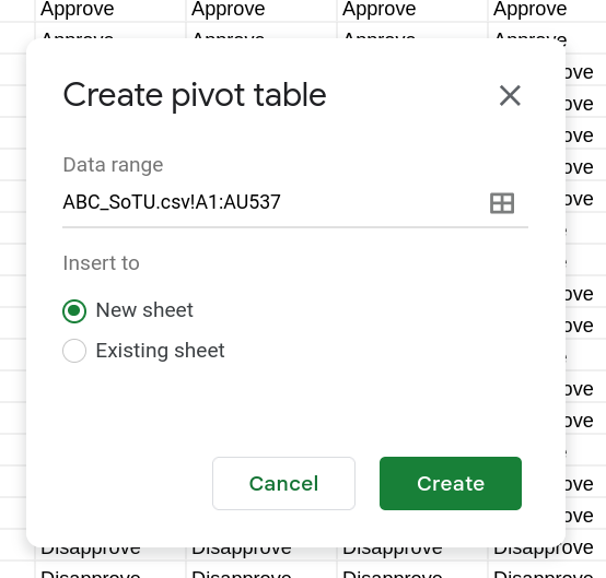
Once you’ve selected Pivot Table a new window will popup (Figure 6). You can use this to change the data that the pivot table will have access to or change where the pivot table is located. For us the defaults work perfectly fine.
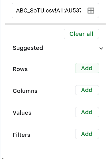
At this point you’ll have a new tab in your Google Sheet (near the bottom) and on the new tab you’ll have your pivot table. On the right side of the new tab you will have a new menu that has opened up (Figure 7). This is where you select variables (columns) that go into your pivot. You can add different variables as rows, values, or as “values”. When you add a variable to the rows (columns) it will use that to create rows (columns) out of the different categories it finds in that variable. The values is used to identify what to calculate in each of those rows (columns). You’ll see that once you select a variable in the values section you’ll have different options on how to use that variable (calculate the average, the sum, standard deviation, etc).
Calculating Proportions
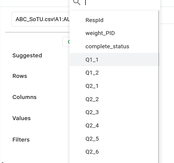
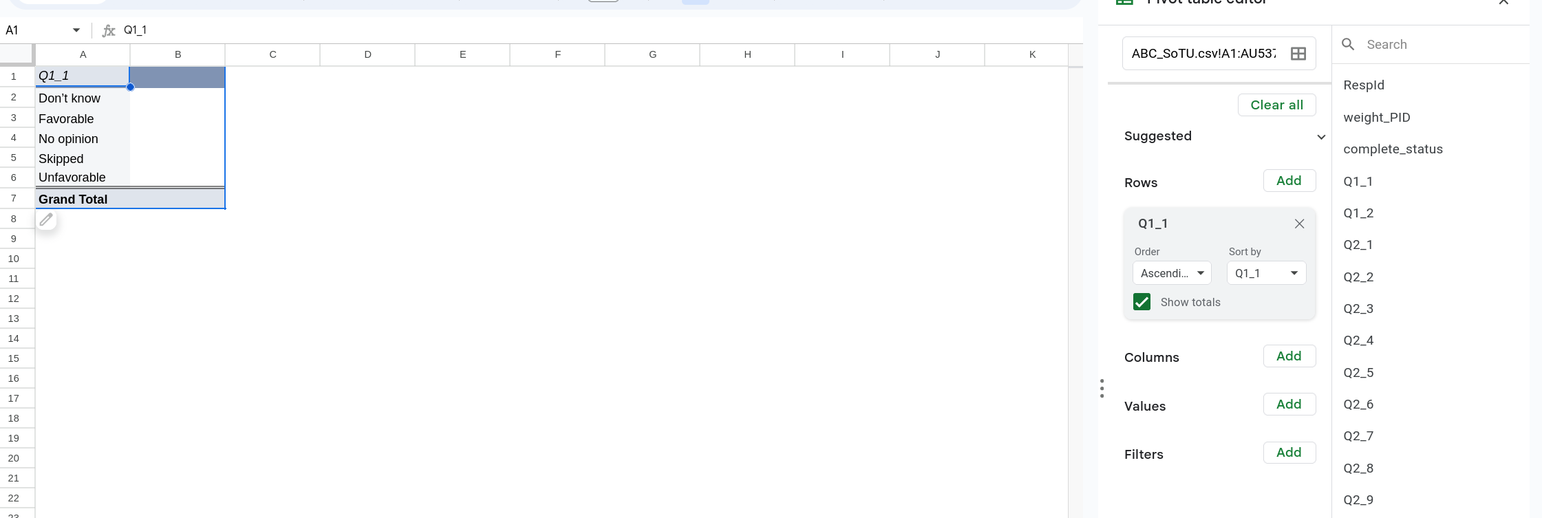
In order to calculate the proportions present in a variable click the Add button next to Rows. A new menu will popup (Figure 8), select the variable you want to use. In this case we are going to pick Q1_1. Once you’ve selected that variable the pivot table will update and you’ll see the different categories listed as different rows (Figure 9).
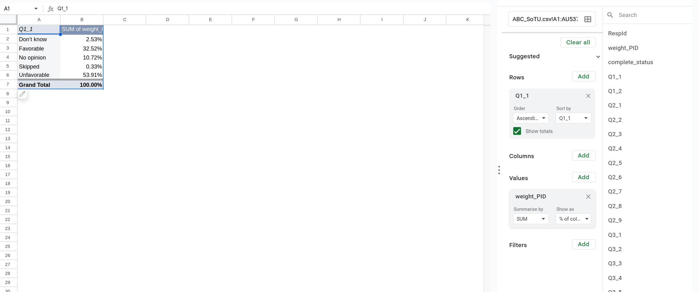
In order to fill in cells we need to add something to the the values. We are going to do this by adding the survey weights. In this case are survey weights are called weight_pid. Click Add next to Values and select weight_PID. By using the weights we adjust how much each individual row counts.1 Once you’ve selected the value it should default to having the Summarize by as SUM. This will sum weight_PID for each row. Finally switch Show as to % of column so that it calculates the percent in each column.
Again what we are doing here is dividing our dataset by whatever we’ve selected in the Row section. We then add up the weight column in each division of the dataset. Finally we convert those sums into proportions/percentages as that’s what we are interested in.
Margin of Error and Confidence Intervals
In order to calculate the Margin of Error and 95% CI we are going to use Google Sheets formulas. These formulas allow you to reference other cells and apply different functions to them. The simplest version would be something like = A5 + B4 which would add the contents of cell A5 to cell B4.
We will start by calculating the standard error. The formula we are using is:
\[ \sqrt{ p(1-p) \frac{N}{N-1} } \]
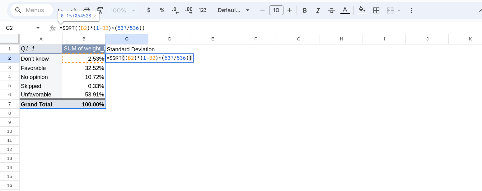
Where \(p\) is the proportion in a category and N is the number of observations in your data. Although it is possible to calculate the number of observations, in this case it is easiest to just note that we have 537 observations. We will pull the proportion directly from the cell.
Start by clicking in the cell where you want the first row’s standard deviation to be. Type = to start a formula. We are going to square root everything so our formula will start with SQRT(. Next we want to click the cell we want to calculate the SD from, this will insert the cell into the formula (you’ll now have something like SQRT(B1). Now multiply that by using the asterisk * by (1-p) by again selecting the cell of interest. Finally multiply that by the number of rows divided by the number of rows minus 1 (putting the latter in parentheses). In full your formula should look something like: SQRT(B1*(1-B1)*(537/536)) (or look at Figure 11).
Once you have the formula you can hit enter and it will calculate the value. It might also suggest filling in the rest of the column with that formula, you can select Ok or do the same thing by clicking down on the blue square in the bottom right corner of the cell and dragging down. When you do this will change the cells you inserted in the formula based on how you drag it. So if you started with B4 and drag down one it will update that to B5. If you dragged it over it will update that to C4.
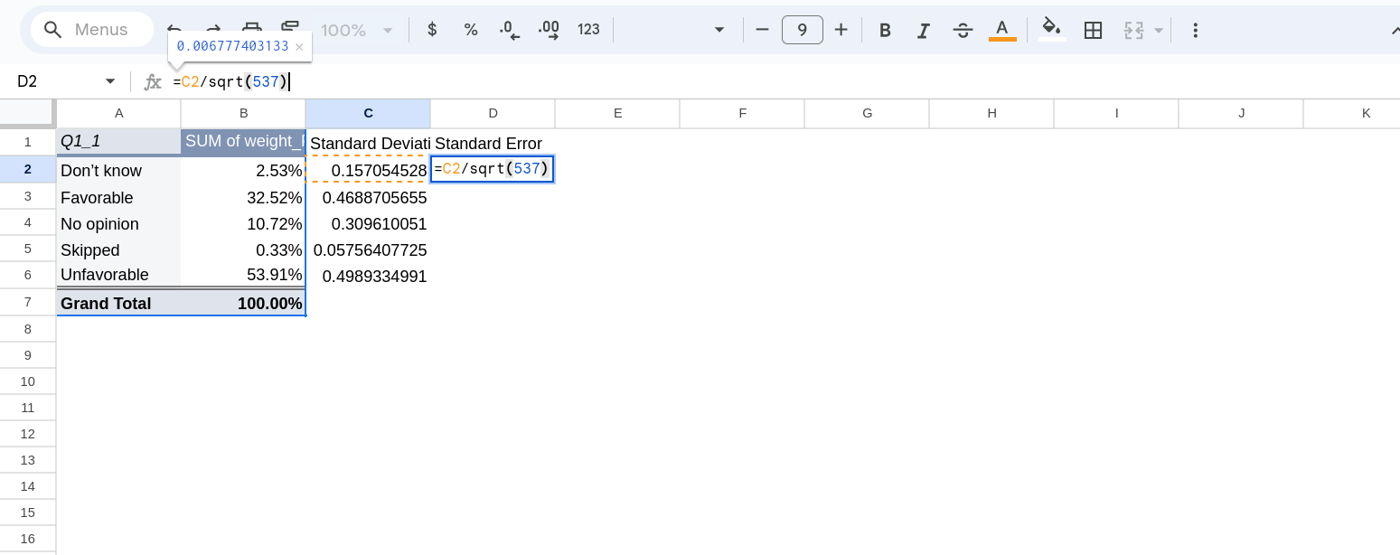
The formula for the standard error is significantly simpler: \(\frac{\sigma}{\sqrt{N}}\). I like to create a column next to the standard deviation with the standard error. You’ll click there type = and then type out your formula. Again drag it down so you have standard errors for everything (Figure 12).
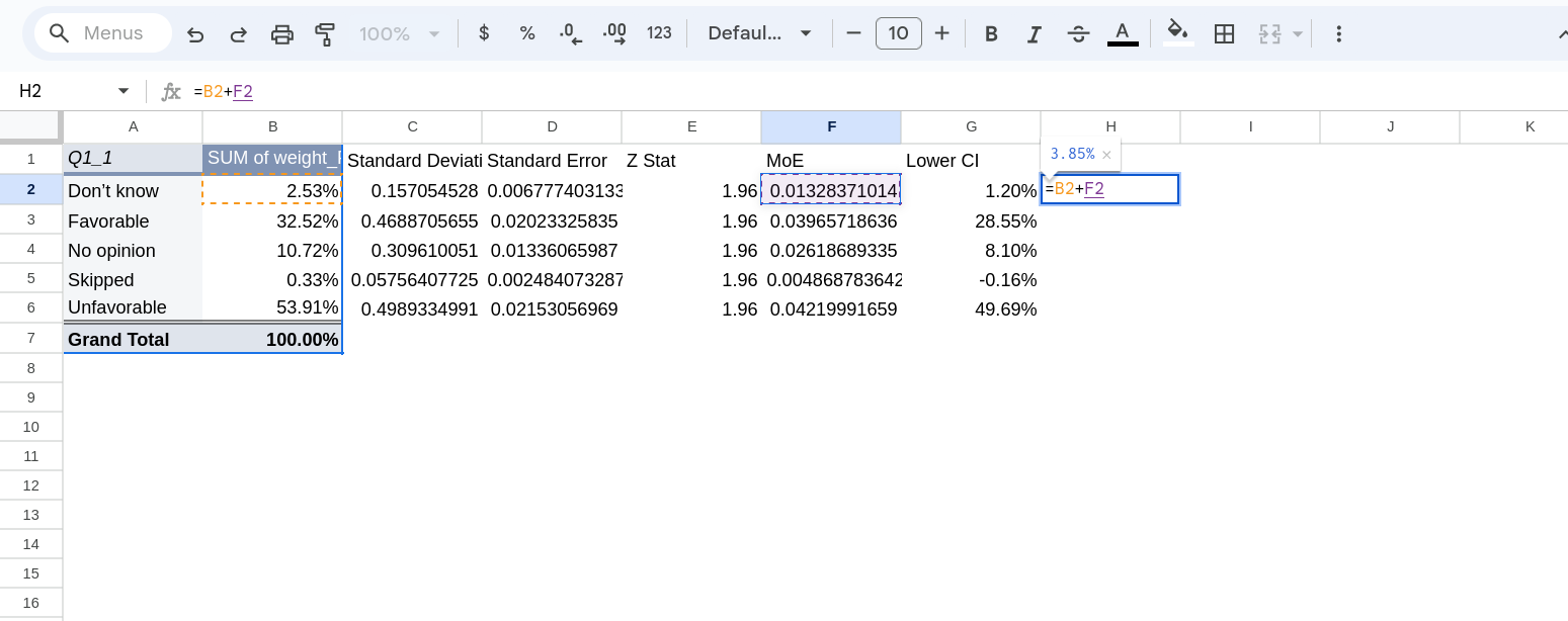
To calculate the margin of error we just multiply the standard error by the relevant Z-stat. For a margin of error related to a 95% CI we use 1.96. I again like to create a column with the relevant Z-stat and then margin of error next to it (Figure 13).

Finally, the bounds of our confidence intervals are calculated by adding/subtracting the margin of error from the raw value. We can again use a formula for this (Figure 14)
Formatting Cells
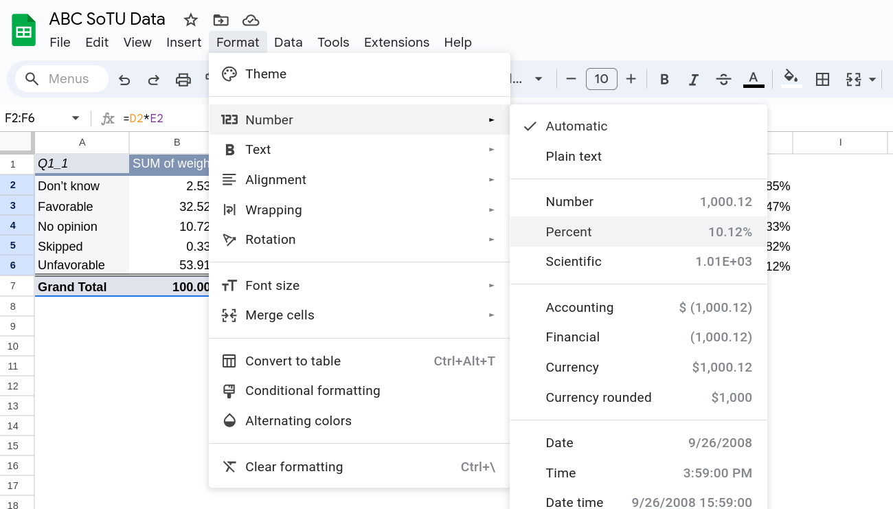
One last thing to note is that we can update how the cells are displayed by highlighting them and selecting Format and the Number and picking Percent from the menu that pops-up (Figure 15). This doesn’t change the underlying values, all it does is change how they are displayed.
Footnotes
If you don’t want to (or don’t have) weights you can select any variable for the values is filled in for every observation and then summarize it by
COUNTA. This option simply counts the number of non-empty cells. You can just use the original variable you used to make the rows, but be careful if you are making crosstabs.↩︎