Cross Tabs in Google Sheets
This guide walks you through how to create cross tabs and calculate a \(\chi^2\) test in Google Sheets. I assume you’ve gone through the guide on calculating univariate statistics which covers how to load a CSV file into a google sheet and create pivot tables.
Creating Cross Tabs
You should again start with a pivot table of your data. Previously we only used the Rows (and values) part of the pivot table, but we are going to now use the Columns options as well. You should select a variable to be along the Rows, the Columns and then add in the weight variable as the Values. In Figure 1 I selected ppeduc5 as the rows, and Q1_1 as the columns (with the correct weights).
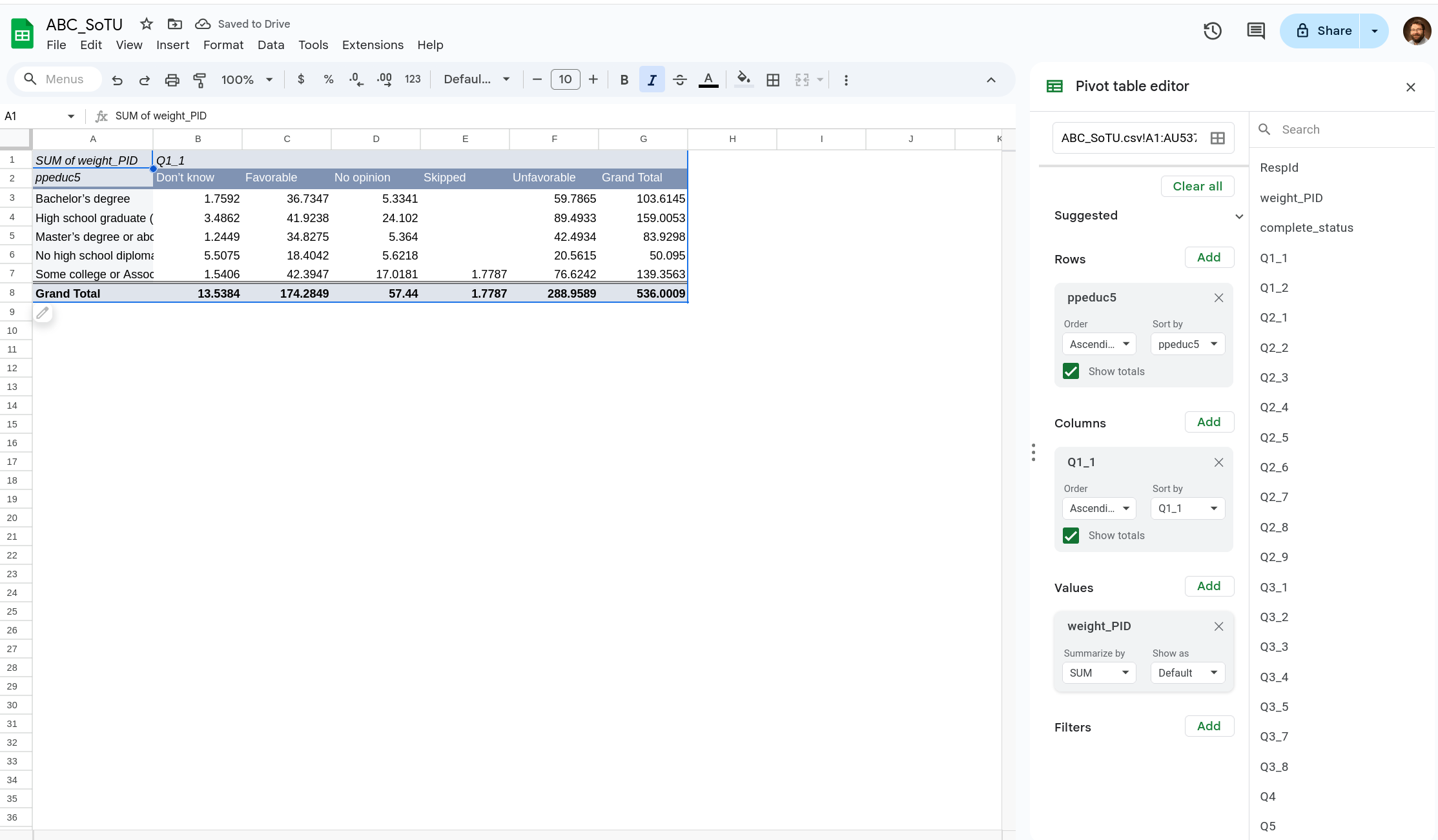
One thing to note is that there were very few people who skipped Q1_1. We probably don’t want to leave it as it is in the table. We have two options, one is to recode those who said “Skip” into something else, another is to just drop the Skip responses. We will do the latter for now.
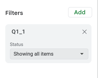
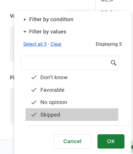
To filter your data use the Filter menu (Figure 2) on the bottom right. You can add a variable to this just like the other menus. I’ve added Q1_1 to it. You can then click on dropdown that appears and select what should (or should not) be shown (Figure 3).
Now we can convert the frequencies into percentages by clicking the Show As option in the Values menu. You can get either row percentages or column percentages using this.
Figure 4 shows the row percentages. This shows, for example, that among those without a high school diploma 10% of them said “Don’t Know” (significantly higher than other groups) and only 41% said they had an unfavorable view of Joe Biden. Joe Biden had the highest unfavorables among those with a bachelor’s degree (57% said they had an unfavorable view of him).
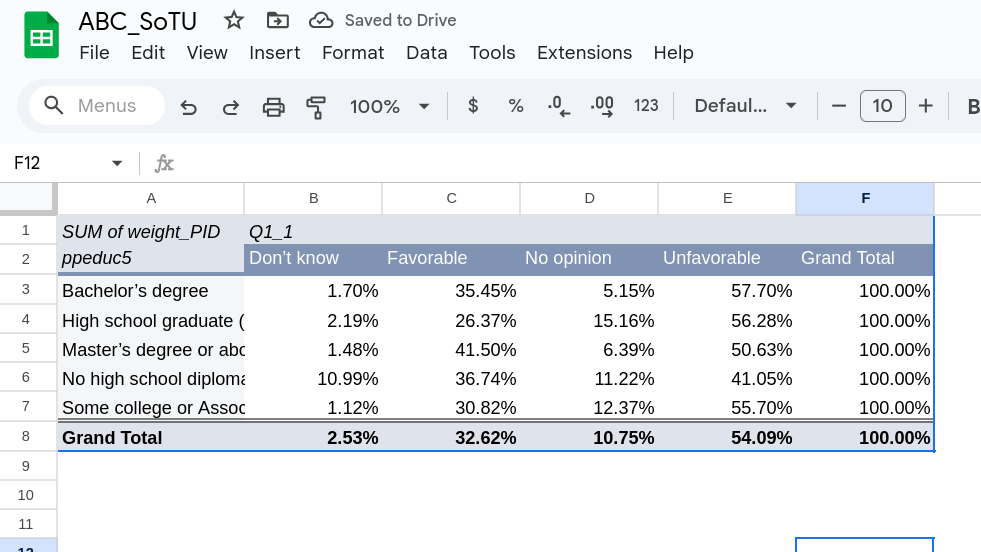
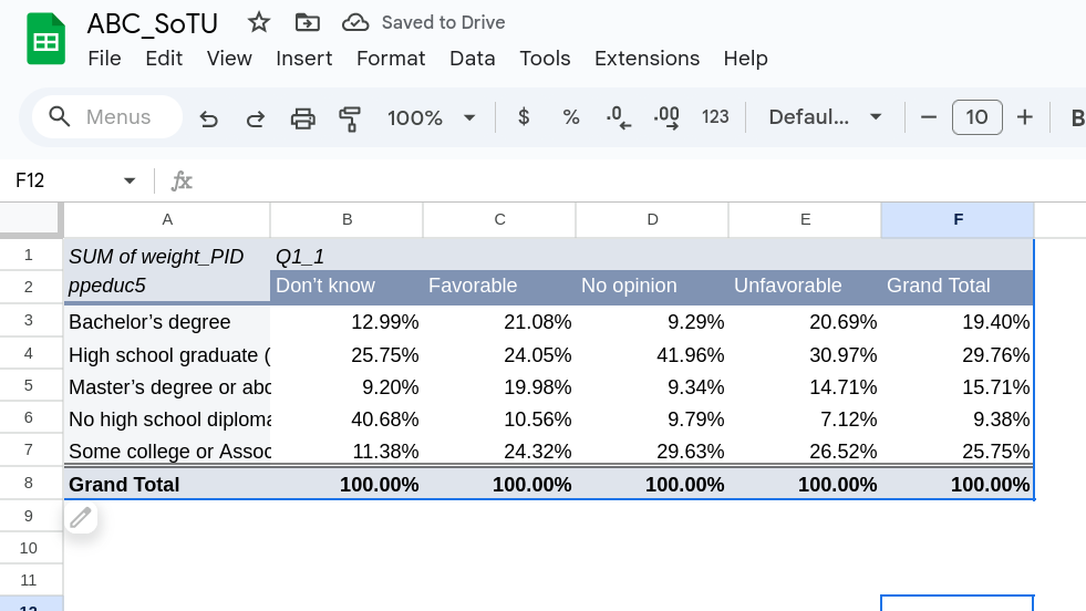
Figure 5 shows the column percentages. Here the data shows that among those who have an unfavorable view of Joe Biden, 31% are high school graduates. Among those who have favorable views, 24% are high school graduates. This might seem weird, but this is because high school graduates were a relatively large portion of the overall sample (the far right column shows this, they made up 30% of the sample).
\(\chi^2\) test
To calculate a \(\chi^2\) test we need to create our observed and expected table. I like to copy this out of the pivot table as it makes it easier to do the google sheets formula. We are going to create the observed table first with both the marginals and the observed frequency. There are several ways to do this but I find it most useful to break this into two steps. Copying the marginals over and then copying over the frequencies for the inner cells.
Observed Table
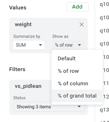
To start go to the Values menu and select “% of Grand Total” from the Show As option (Figure 6). This calculates each cell as the percentage for the whole table, which makes the bottom row and far column the marginals.
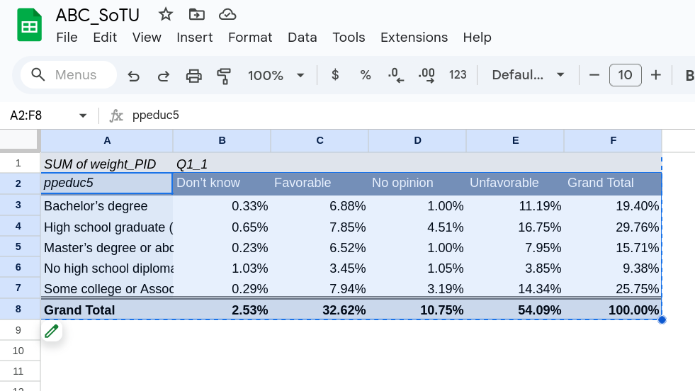
Once you do this you should have a table thats look like Figure 7. We are going to highlight the pivot table to copy the information out of it.
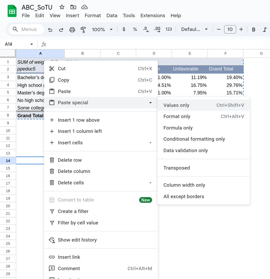
Now right click somewhere below the table and select “Paste special” and then “Values.” This will paste just the contents of the cells opposed to also pasting the formatting or equations (Figure 8)
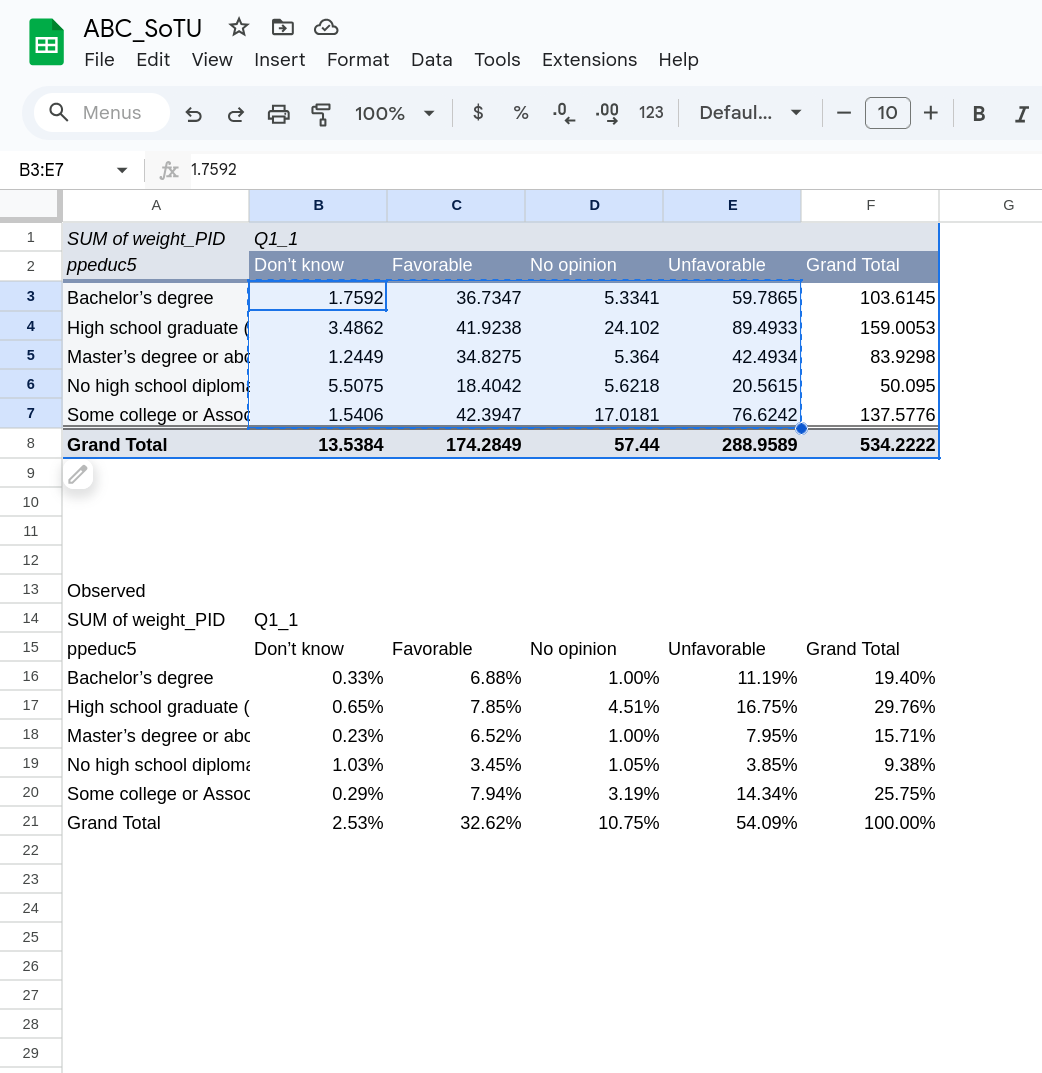
Now go back to the pivot table and switch it from “% of Grand Total” back to “Default”. Now we have the frequencies only. Highlight just the inside cells of the table (see Figure 9) and copy that part.
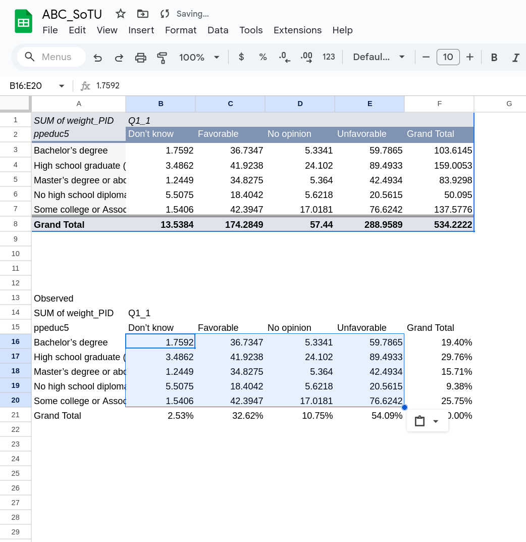
Then go down to what copied before and highlight the same area in that new table and paste in what you just copied. You should again go to “Paste special” and then “Values”. You should now have something that looks like Figure 10.
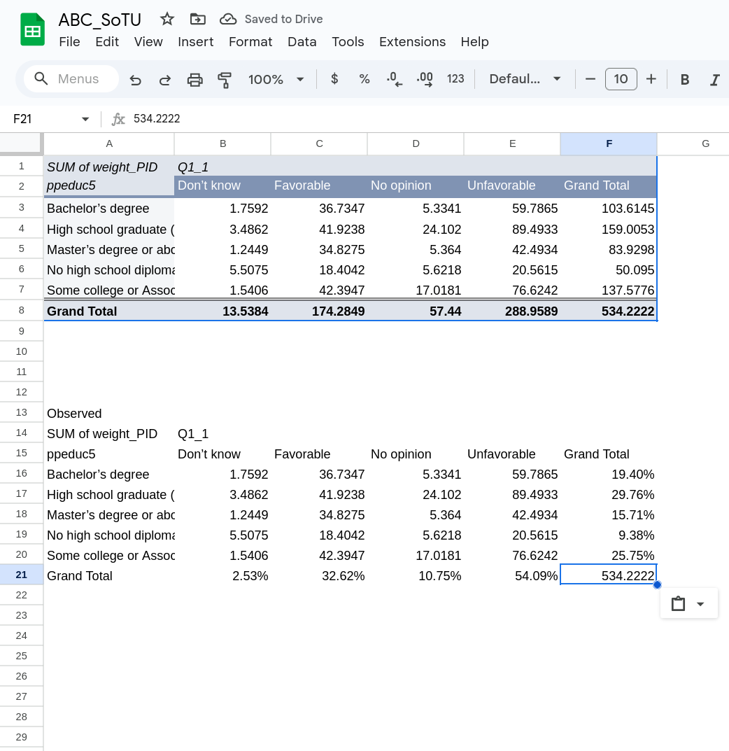
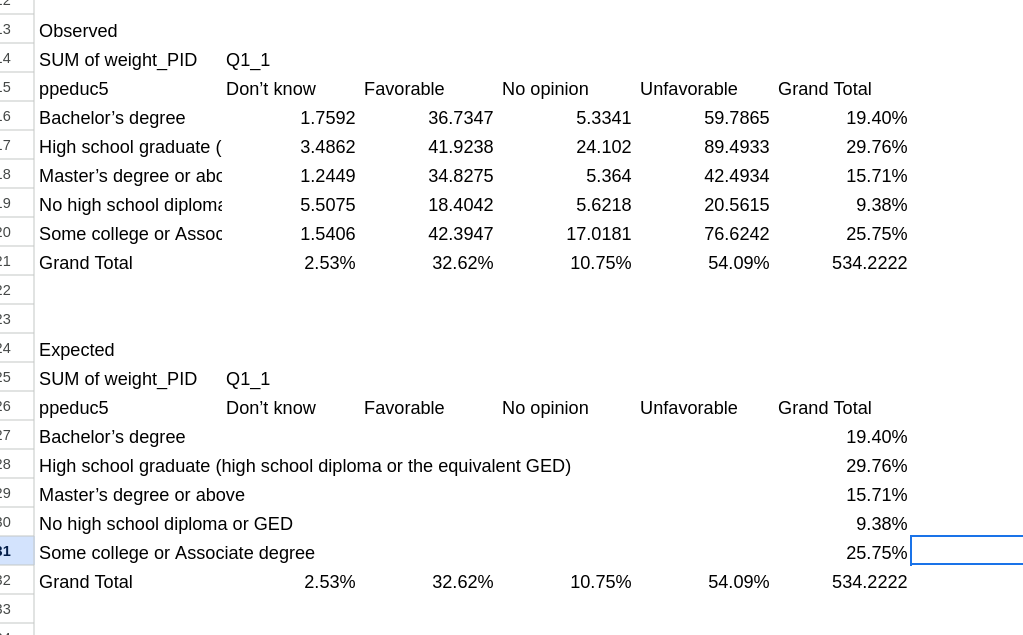
As a final step, copy the Grand Total down from the pivot table into this table. Your final table will have frequencies in the inside, margins on the bottom and right, and then the total number of observations in the bottom right cell.
Expected Table
Now we are going to create a table where we will put in our expectations under the assumption of independence. We can start with by copying the entire observed table and putting the expected table somewhere below it. I find it helpful to label both. You can then delete all the cells in the center of your newly created expected table. You should now have something that looks like Figure 12.
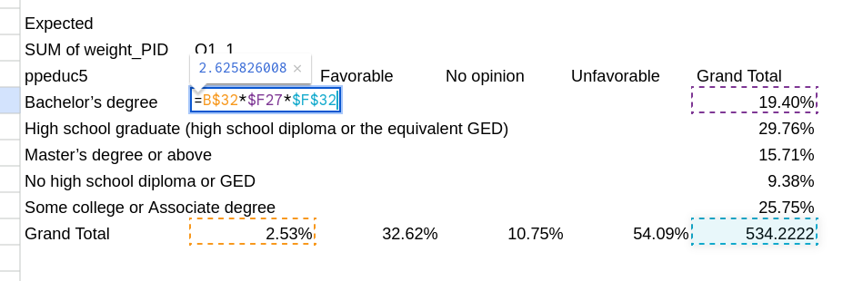
Remember, the expected value of each cell in this new table with be the row marginal multiplied by the column marginal multiplied by the total number of observations. We will again use some formulas to do that, but we are going to make it easier for us to drag the formula to other spots in the table.
We will start in the top left of the expected table, and we will want to reference the furthest left margin and the top row margin. So in this case we could type =B32 * F27 * F32 in the formula and be correct. The problem though is that we want to drag this formula over to the other cells. If we drag this one to the right we’d get = C32 * G27 * G32 which wouldn’t be right. We want to freeze some of this formula. To do that we we use a $ in front of the part we don’t want to move. So we will instead type: =B$32 * $F27 * $F$32 This freezes the first as staying within the row margin, the second as staying within the column margin and the third as staying in the bottom right corner. To see this in action look at Figure 13
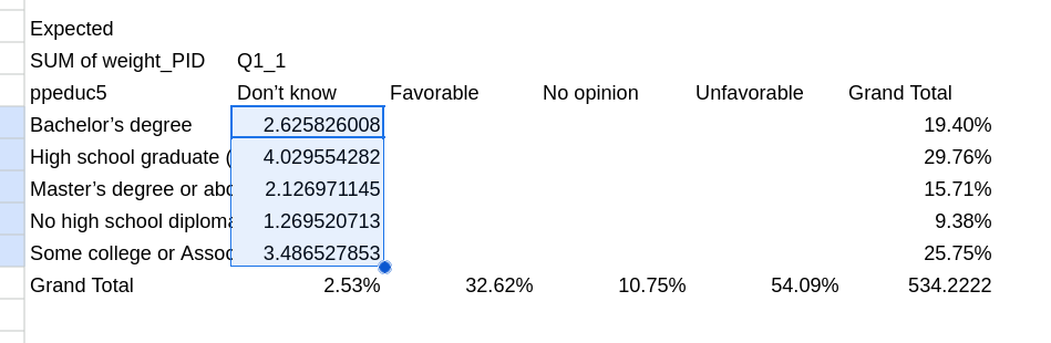
Now that you have that formula in you can click on it and drag it down (Figure 14). Then highlight it all and drag it to the right (Figure 15)
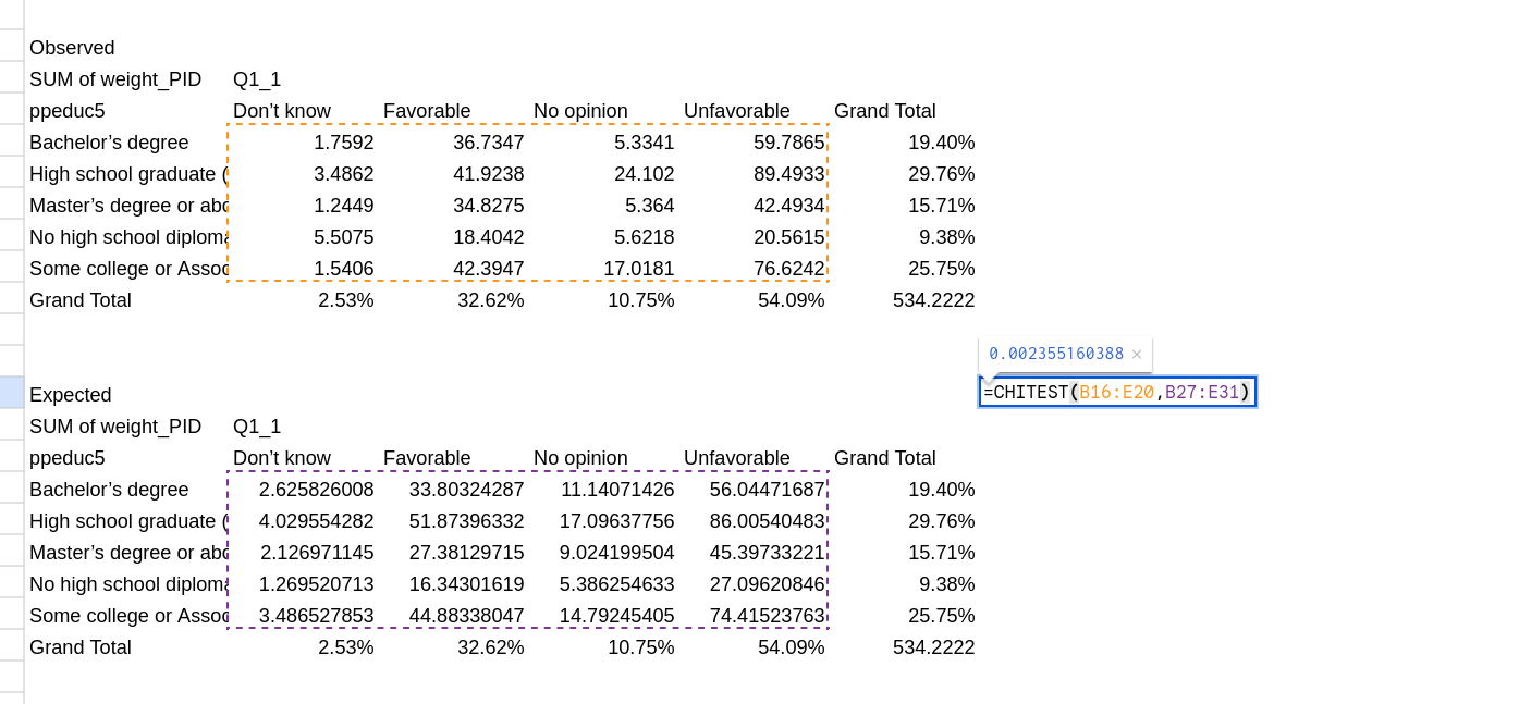
Calculating your p-value
Finally we can calculate our p-value directly from these tables. We will use the CHITEST() function which takes in two arguments: the observed table and the expected table. You should start by typing =CHITEST( into a cell. You can then click and highlight the observed table and hit enter. Next click and highlight the expected table and hit enter. You should get something that looks like Figure 16. Once you click off the cell you’ll get your p-value.